NOTE: This page was developed using G*Power version 3.1.9.2. You can download the current version of G*Power from https://www.psychologie.hhu.de/arbeitsgruppen/allgemeine-psychologie-und-arbeitspsychologie/gpower.html. You can also find help files, the manual and the user guide on this website.
Introduction
Power analysis is the name given to the process for determining the sample size for a research study. The technical definition of power is that it is the probability of detecting a “true” effect when it exists. Many students think that there is a simple formula for determining sample size for every research situation. However, the reality is that there are many research situations that are so complex that they almost defy rational power analysis. In most cases, power analysis involves a number of simplifying assumptions, in order to make the problem tractable, and running the analyses numerous times with different variations to cover all of the contingencies.
In this unit we will try to illustrate how to do a power analysis for multiple regression model that has two control variables, one continuous research variable and one categorical research variable (three levels).
Description of the experiment
A school district is designing a multiple regression study looking at the effect of gender, family income, mother’s education and language spoken in the home on the English language proficiency scores of Latino high school students. The variables gender and family income are control variables and not of primary research interest. Mother’s education is a continuous variable that measures the number of years that the mother attended school. The range of this variable is expected to be from 4 to 20. The variable language spoken (homelang) in the home is a categorical research variable with three levels: 1) Spanish only, 2) both Spanish and English, and 3) English only. Since there are three levels, it will take two dummy variables to code language spoken in the home.
The full regression model will look something like this:
engprof = b0 + b1(gender) + b2(income) + b3(momeduc) + b4(homelang1) + b5(homelang2)
Thus, the primary research hypotheses are the test of b3 and the joint test of b4 and b5. These tests are equivalent the testing the change in R2 when momeduc (or homelang1 and homelang2) are added last to the regression equation.
The power analysis
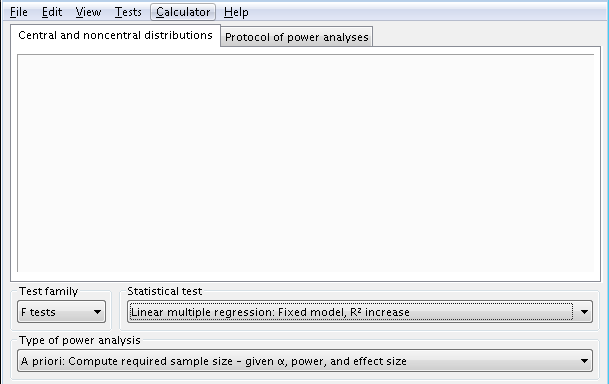
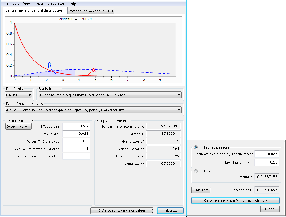
Let’s set up the analysis. Under Test family select F tests, and under Statistical test select ‘Linear multiple regression: Fixed model, R2 increase’. Under Type of power analysis, choose ‘A priori…’, which will be used to identify the sample size required given the alpha level, power, number of predictors and effect size.
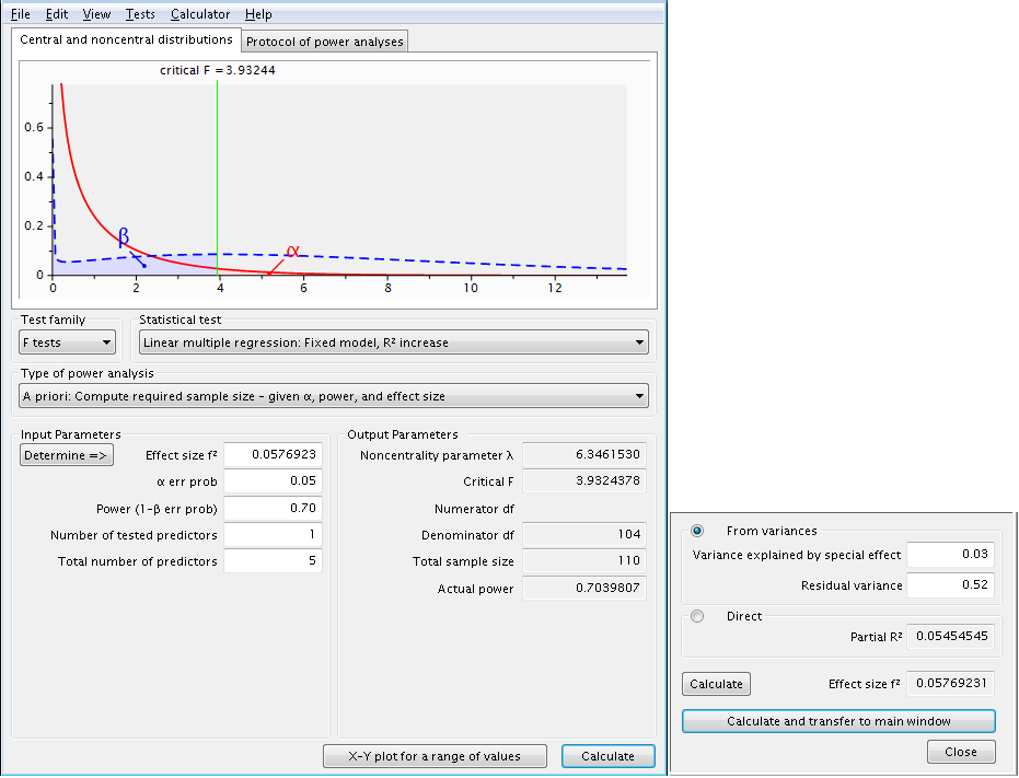
The latter can be determined via the ‘Determine =>’ button, which calls up a menu requesting the variance explained by the special effect and the residual variance.
We believe, from previous research, that the R2 for the full-model with five predictor variables (2 controls, 1 continuous research, and 2 dummy variables for the categorical variable) will be will be about 0.48.
Let’s start with the continuous predictor (momeduc, the special effect in this case). We think that it will add about 0.03 to the R2 when it is added last to the model. This is what we put under ‘Variance explained by special effect’.
The residual variance is defined as 1 – (R2 of the full-model), and in this case is 1 – 0.48 = 0.52. The total number of variables (predictors) is 5 and the number being tested (df) is one. Let’s assume that the power is 0.70.
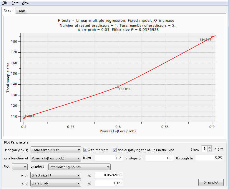
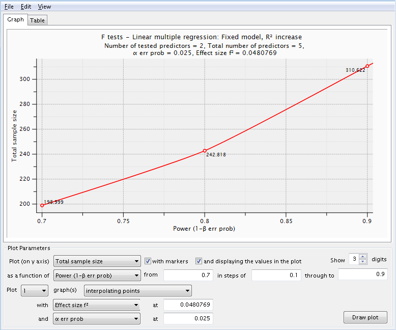
We will run three calculations with power equal to 0.7, 0.8 and 0.9. Making use of the ‘X-Y plot for a range of values’ button and denoting power as the independent variable y ranging from 0.7 to 0.9 in steps of 0.1:
This gives us a range of sample sizes ranging from 109 to 184 depending on power.
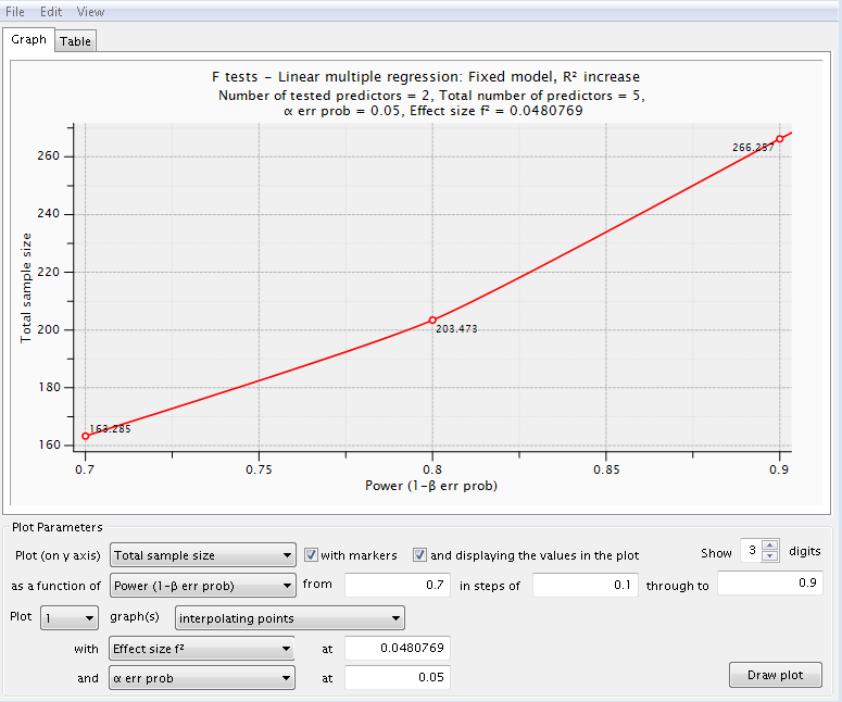
Let’s see how this compares with the categorical predictor (homelang1 and homelang2) which uses two dummy variables in the model. We believe that the change in R2 (variance explained by the special effect) attributed to the two dummy variables will be about 0.025. Note that the residual variance is still defined as 1 – 0.48 = 0.52 so this does not change. The total number of predictors stays at 5 while the numerator df (number of tested predictors) is now 2.
This series of power analyses yielded sample sizes ranging from 163 to 266. These sample sizes are larger than those for the continuous research variable.
If it is the case that both of these research variables are important, we might want to take into that we are testing two separate hypotheses (one for the continuous and one for the categorical) by adjusting the alpha level. The simplest but most draconian method would be to use a Bonferroni adjustment by dividing the nominal alpha level, 0.05, by the number of hypotheses, 2, yielding an alpha of 0.025. We will rerun the categorical variable power analysis using the new adjusted alpha level.
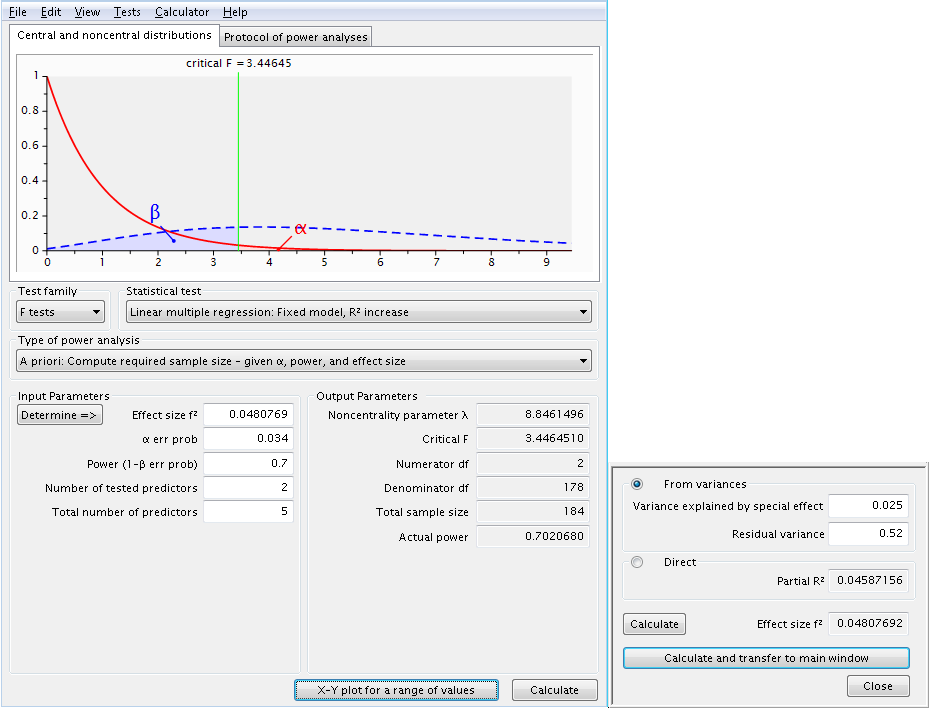
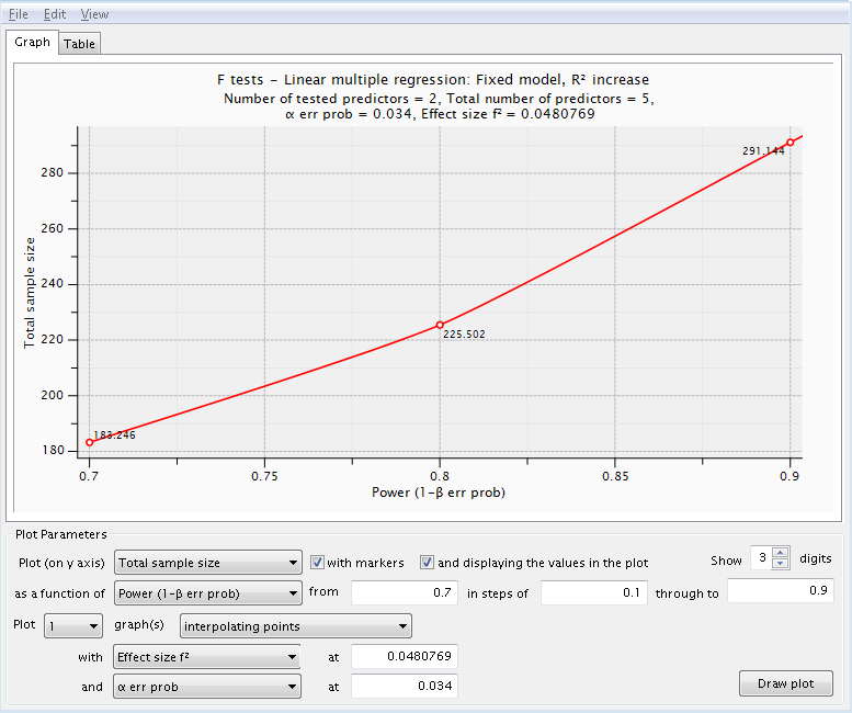
The Bonferroni adjustment assumes that the tests of the two hypotheses are independent which is, in fact, not the case. The squared correlation between the two sets of predictors is about .2 which is equivalent to a correlation of approximately .45. Using an internet applet to compute a Bonferroni adjusted alpha taking into account the correlation gives us an adjusted alpha value of 0.034 to use in the power analysis.
Based on the series of power analyses the school district has decided to collect data on a sample of about 225 students. This sample size should yield a power of around 0.8 in testing hypotheses concerning both the continuous research (momeduc) variable and the categorical research variable, language spoken in the home (homelang1 and homelang2). The nominal alpha level is 0.05 but has been adjusted to .034 to take into account the number of hypotheses tested and the correlation between the predictors.

