
Version info: Code for this page was tested in Mplus version 6.12.
Negative binomial regression is used to model count variables with
overdispersion.
Please note: The purpose of this page is to show how to use various data
analysis commands. It does not cover all aspects of the research process which
researchers are expected to do. In particular, it does not cover data
cleaning and checking, verification of assumptions, model diagnostics or
potential follow-up analyses.
Examples of negative binomial regression
Example 1. School administrators study the attendance behavior of high school juniors at two schools.
Predictors of the number of days of absence include the type of program in which
the student is enrolled and a standardized
test in math.
Example 2. A health-related researcher is studying the number of
hospital visits in past 12 months by senior citizens in a community based on the
characteristics of the individuals and the types of health plans under which
each one is covered.
Description of the data
We have attendance data on 314 high school juniors from two urban high schools in
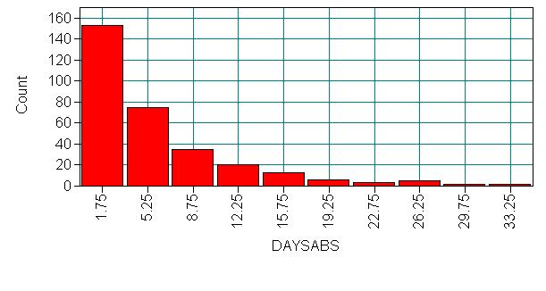
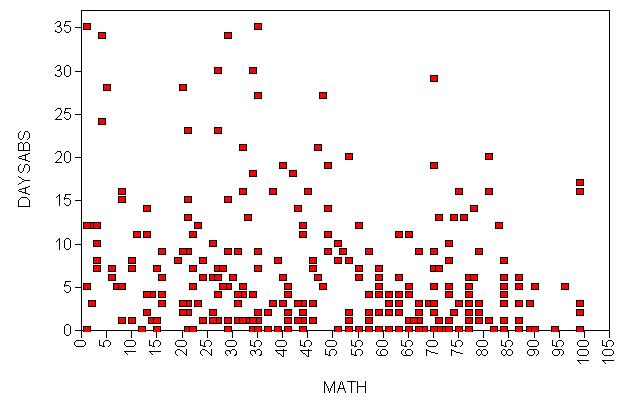
the file https://stats.idre.ucla.edu/wp-content/uploads/2016/02/nb_data.dat. The response variable of interest is days absent, daysabs.
The variable math gives the standardized math score for
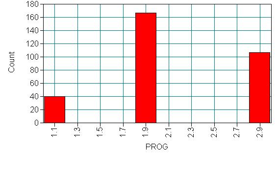
each student. The variable prog is a three-level nominal variable
indicating the type of instructional program in which the student is enrolled.
The variables p1, p2 and p3 are dummy-coded indicator variables
for prog.
Let’s look at the data. It is always a good idea to start with descriptive
statistics.
Data:
File is g:daehttps://stats.idre.ucla.edu/wp-content/uploads/2016/02/nb_data.dat;
Variable:
Names are
id gender math daysabs prog p1 p2 p3;
Missing are all (-9999);
usevariables are id gender math daysabs prog p1 p2 p3;
analysis:
type = basic;
plot: type is plot1;
RESULTS FOR BASIC ANALYSIS

ESTIMATED SAMPLE STATISTICS


           Means
              ID            GENDER        MATH          DAYSABS       PROG
              ________      ________      ________      ________      ________
      1      1575.911         1.490        48.268         5.955         2.213


           Means
              P1            P2            P3
              ________      ________      ________
      1         0.127         0.532         0.341


           Covariances
              ID            GENDER        MATH          DAYSABS       PROG
              ________      ________      ________      ________      ________
 ID        251516.623
 GENDER       -27.319         0.250
 MATH        4840.852        -0.227       641.202
 DAYSABS    -1193.221        -0.357       -41.966        49.361
 PROG         165.742         0.004         3.895        -1.717         0.423
 P1           -17.479        -0.005        -0.439         0.598        -0.155
 P2          -130.784         0.007        -3.018         0.521        -0.113
 P3           148.263        -0.002         3.457        -1.119         0.268


           Covariances
              P1            P2            P3
              ________      ________      ________
 P1             0.111
 P2            -0.068         0.249
 P3            -0.043        -0.181         0.225


           Correlations
              ID            GENDER        MATH          DAYSABS       PROG
              ________      ________      ________      ________      ________
 ID             1.000
 GENDER        -0.109         1.000
 MATH           0.381        -0.018         1.000
 DAYSABS       -0.339        -0.102        -0.236         1.000
 PROG           0.508         0.011         0.237        -0.376         1.000
 P1            -0.105        -0.031        -0.052         0.255        -0.713
 P2            -0.523         0.027        -0.239         0.148        -0.350
 P3             0.624        -0.006         0.288        -0.336         0.870


           Correlations
              P1            P2            P3
              ________      ________      ________
 P1             1.000
 P2            -0.407         1.000
 P3            -0.275        -0.766         1.000
Analysis methods you might consider
Below is a list of some analysis methods you may have
encountered. Some of the methods listed are quite reasonable, while others have
either fallen out of favor or have limitations.
- Negative binomial regression -Negative binomial regression can be used
for over-dispersed count data, that is when the conditional variance exceeds
the conditional mean. It can be considered as a generalization of Poisson
regression since it has the same mean structure as Poisson regression and it
has an extra parameter to model the over-dispersion. If the conditional
distribution of the outcome variable is over-dispersed, the confidence
intervals for the Negative binomial regression are likely to be narrower as
compared to those from a Poisson regression model. - Poisson regression – Poisson regression is often used for modeling count
data. Poisson regression has a number of extensions useful for count models. - Zero-inflated regression model – Zero-inflated models attempt to account
for excess zeros. In other words, two kinds of zeros are thought to
exist in the data, "true zeros" and "excess zeros". Zero-inflated
models estimate two equations simultaneously, one for the count model and one for the
excess zeros. - OLS regression – Count outcome variables are sometimes log-transformed
and analyzed using OLS regression. Many issues arise with this
approach, including loss of data due to undefined values generated by taking
the log of zero (which is undefined), as well as the lack of capacity to
model the dispersion.
Negative binomial regression analysis
In the Mplus syntax below, we specify that the variables to be used in the
negative binomial regression are daysabs, math, p2, p3,
which will make prog=1 the reference group. We also specify that daysabs is a count variable, and we include (nb)
to indicate that we want a negative binomial regression. (By default,
Mplus would model this as a Poisson regression.) By
default, Mplus uses restricted maximum likelihood (MLR), so robust standard
errors would be given in the output. Here, the standard errors are calculated using
maximum likelihood estimates by including the analysis: estimator = ml; block.
Data:
File is g:daehttps://stats.idre.ucla.edu/wp-content/uploads/2016/02/nb_data.dat;
Variable:
Names are
id gender math daysabs prog p1 p2 p3;
Missing are all (-9999);
usevariables are daysabs math p2 p3;
count is daysabs (nb);
model:
daysabs on math p2 p3;
analysis: estimator = ml;

MODEL FIT INFORMATION

Number of Free Parameters                        5

Loglikelihood

          H0 Value                        -865.629

Information Criteria

          Akaike (AIC)                    1741.258
          Bayesian (BIC)                  1760.005
          Sample-Size Adjusted BIC        1744.146
            (n* = (n + 2) / 24)


MODEL RESULTS

                                                    Two-Tailed
                    Estimate       S.E.  Est./S.E.    P-Value

 DAYSABS    ON
    MATH              -0.006      0.003     -2.390      0.017
    P2                -0.441      0.183     -2.414      0.016
    P3                -1.279      0.202     -6.331      0.000

 Intercepts
    DAYSABS            2.615      0.196     13.319      0.000

 Dispersion
    DAYSABS            0.968      0.100      9.729      0.000
- After the heading informing that "THE MODEL ESTIMATION TERMINATED NORMALLY"
comes the information about the model. It begins with the information
regarding the log likelihood, AIC and BIC. These can be used in comparing models. - Then we will find the
negative binomial regression coefficients for each of the variables along with the
standard errors. The column labeled as Est./S.E. is the quotient of the estimates divided by
the standard errors. These are basically z-scores if the sample size is reasonably large. In the right-most column
is the two-tailed p-value. - The variable math has a coefficient of -0.006, which
is statistically significant. This means that for each one-unit
increase on math, the expected log count of the number of days absent
decreases by 0.006 day. Both of the dummy variables for the variable
prog are statistically significant. Compared to level 1 of
prog, the expected log count for level 2 decreases by 0.441.
Compared to level 1 of prog, the expected log count of for level 3
decreases by 1.279. - Additionally, under "Dispersion" we find the estimate of the natural log of the
over-dispersion coefficient, alpha. If the alpha coefficient is zero then
the model is better estimated using a Poisson regression
model. Here it is different from zero, so negative binomial regression is
appropriate.
To determine if prog itself is statistically significant, we can
use the model test block to obtain the two degree-of-freedom test of this
variable. Additionally, we can get an estimate of the natural log of the
over-dispersion coefficient, alpha. If the alpha coefficient is zero then
the model is better estimated using a Poisson regression model.
Data:
File is g:daehttps://stats.idre.ucla.edu/wp-content/uploads/2016/02/nb_data.dat;
Variable:
Names are
id gender math daysabs prog p1 p2 p3;
Missing are all (-9999);
usevariables are daysabs math p2 p3;
count is daysabs (nb);
model:
daysabs on
math (a1)
p2 (a2)
p3 (a3);
model test:
a2 = 0;
a3 = 0;
analysis: estimator = ml;
MODEL FIT INFORMATION<**SOME OUTPUT OMITTED**> Wald Test of Parameter Constraints Value 49.214 Degrees of Freedom 2 P-Value 0.0000
In the syntax above, some of the variables in the model are given labels.
These labels must be in parentheses and must be the last item listed on the
line, so the model is broken up over several lines. We have given the
label a2 to the indicator variable p2, and the label a3 to
the indicator variable p3. Once we have assigned labels to the
variables, we can use those labels in the model test block.
Setting both a2 and a3 to 0 allows us to get the two
degree-of-freedom test of the variable prog. We can see that the
variable prog, as a whole, is statistically significant.
To obtain the results as incident rate ratios, we need to use the model
constraint block. Again, we use labels to refer to the variables
in the model. In the model constraint block, we use the new
statement to label the new parameters, which will be the exponentiated
parameters from the model.
Data:
File is g:daehttps://stats.idre.ucla.edu/wp-content/uploads/2016/02/nb_data.dat;
Variable:
Names are
id gender math daysabs prog p1 p2 p3;
Missing are all (-9999);
usevariables are daysabs math p2 p3;
count is daysabs (nb);
model:
daysabs on
math (a1)
p2 (a2)
p3 (a3);
model constraint:
new( math_exp p2_exp p3_exp);
math_exp = exp(a1);
p2_exp = exp(a2);
p3_exp = exp(a3);
analysis: estimator = ml;

MODEL FIT INFORMATION

Number of Free Parameters                        5

Loglikelihood

          H0 Value                        -865.629

Information Criteria

          Akaike (AIC)                    1741.258
          Bayesian (BIC)                  1760.005
          Sample-Size Adjusted BIC        1744.146
            (n* = (n + 2) / 24)


MODEL RESULTS

                                                    Two-Tailed
                    Estimate       S.E.  Est./S.E.    P-Value

 DAYSABS    ON
    MATH              -0.006      0.003     -2.390      0.017
    P2                -0.441      0.183     -2.414      0.016
    P3                -1.279      0.202     -6.331      0.000

 Intercepts
    DAYSABS            2.615      0.196     13.319      0.000

 Dispersion
    DAYSABS            0.968      0.100      9.729      0.000

 New/Additional Parameters
    MATH_EXP           0.994      0.002    398.851      0.000
    P2_EXP             0.644      0.117      5.477      0.000
    P3_EXP             0.278      0.056      4.951      0.000
Things to consider
- It is not recommended that negative binomial models be applied to small
samples. - One common cause of over-dispersion is excess zeros by an additional
data generating process. If
more than one process generates the data, then it is possible to have more
0s than expected by the negative binomial model; in this case, a zero-inflated model (either zero-inflated Poisson or
zero-inflated negative binomial) may be more appropriate. - If the data generating process does not allow for any 0s (such as the
number of days spent in the hospital), then a zero-truncated model may be
more appropriate. - Count data often have an exposure variable, which indicates the number
of times the event could have happened. This variable can be
incorporated into your negative binomial model by taking the log of the
exposure variable and constraining its estimate to 1. - The outcome variable in a negative binomial regression cannot have negative numbers, and the exposure
cannot have 0s. - Pseudo-R-squared: Many different measures of pseudo-R-squared exist. They all attempt to provide information similar to
that provided by R-squared in OLS regression; however, none of them can be interpreted exactly as R-squared in OLS regression
is interpreted. For a discussion of various pseudo-R-squares, see Long and Freese (2006) or our FAQ page What are pseudo
R-squareds? .
See also
References
- Long, J. S. 1997. Regression Models for Categorical and Limited Dependent Variables.
Thousand Oaks, CA: Sage Publications. - Long, J. S. and Freese, J. 2006. Regression Models for
Categorical Dependent Variables Using Stata, Second Edition.
College Station, TX: Stata Press. - Cameron, A. C. and Trivedi, P. K. 2009. Microeconometrics Using
Stata. College Station, TX: Stata Press. - Cameron, A. C. and Trivedi, P. K. 1998. Regression
Analysis of Count Data. New York: Cambridge Press. - Cameron, A. C. Advances in Count Data Regression Talk for the
Applied Statistics Workshop, March 28, 2009.
http://cameron.econ.ucdavis.edu/racd/count.html . - Dupont, W. D. 2002. Statistical Modeling for Biomedical
Researchers: A Simple Introduction to the Analysis of Complex Data.
New York: Cambridge Press.