
Version Info: Code for this page was tested in Mplus
version 6.12.
Please note: The purpose of this page is to show how to use various data analysis commands.
It does not cover all aspects of the research process which researchers are expected to do. In
particular, it does not cover data cleaning and checking, verification of assumptions, model
diagnostics and potential follow-up analyses.
Examples of ordered logistic regression
Example 1: A marketing research firm wants to
investigate what factors influence the size of soda (small, medium, large or
extra large) that people order at a fast-food chain. These factors may
include what type of sandwich is ordered (burger or chicken), whether or not
fries are also ordered, and age of the consumer. While the outcome
variable, size of soda, is obviously ordered, the difference between the various
sizes is not consistent. The differece between small and medium is 10
ounces, between medium and large 8, and between large and extra large 12.
Example 2: A researcher is interested in what factors influence medaling
in Olympic swimming. Relevant predictors include at training hours, diet,
age, and popularity of swimming in the athlete’s home country. The
researcher believes that the distance between gold and silver is larger than the
distance between silver and bronze.
Example 3: A study looks at factors that influence the decision of
whether to apply to graduate school. College juniors are asked if they are
unlikely, somewhat likely, or very likely to apply to graduate school.
Hence, our outcome variable has three categories. Data on parental educational status, whether the undergraduate institution is
public or private, and current GPA is also collected. The
researchers have reason to believe that the “distances” between these three
points are not equal. For example, the “distance” between “unlikely” and
“somewhat likely” may be shorter than the distance between “somewhat likely” and
“very likely”.
Description of the Data
For our data analysis below, we are going to expand on Example 3 about
applying to graduate school. We have generated hypothetical data,
which can be obtained here.
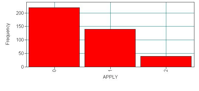
This hypothetical data set has a thee level variable called apply
(coded 0, 1, 2), that we will use as our response (i.e., outcome, dependent)
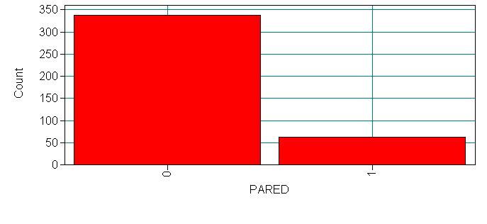
variable. We also have three variables that we will use as predictors: pared,
which is a 0/1 variable indicating whether at least one parent has a graduate degree;
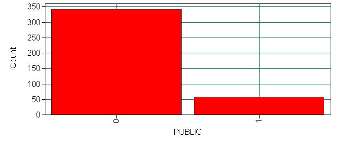
public, which is a 0/1 variable where 1 indicates that the undergraduate
institution is a public university and 0 indicates that it is a private university,
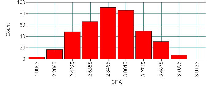
and gpa, which is the student’s grade point average. Let’s start with some
descriptive statistics for the variables of interest.
  Title: Ordinal logistic regression in Mplus;
  Data:
    File is D:documentsologit in Mplus DAEologit.dat ;
  Variable:
    Names are apply pared public gpa;
      categorical are apply;
  Analysis:
    type = basic;
  Plot:
    type = plot1;
For this output only, we will display all of the information in the output.
You will want to look at this carefully to be sure that the data were read into
Mplus correctly. You will want to make sure that you have the correct number
of observations, and that the categorical and continuous variables have been
correctly specified. We have not used a missing statement because we have no
missing data in this data set. If any of our variables had missing data we would
have specified “missing = #” in the variable statement,
where # is the numeric value given to missing values (e.g. -9999). Below the
output are histograms for each of our four variables, these were produced using
the plotting function in Mplus. In order to be able to do this, we included the
plot statement and specified “type = plot1” which tells Mplus to create
the auxiliary files necessary for the plotting function.
INPUT READING TERMINATED NORMALLY

Ordinal logistic regression in Mplus;

SUMMARY OF ANALYSIS

Number of groups                                                 1
Number of observations                                         400

Number of dependent variables                                    4
Number of independent variables                                  0
Number of continuous latent variables                            0

Observed dependent variables

  Continuous
   PARED       PUBLIC      GPA

  Binary and ordered categorical (ordinal)
   APPLY


Estimator                                                    WLSMV
Maximum number of iterations                                  1000
Convergence criterion                                    0.500D-04
Maximum number of steepest descent iterations                   20
Parameterization                                             DELTA

Input data file(s)
  D:documentsologit in Mplus DAEologit.dat

Input data format  FREE


SUMMARY OF CATEGORICAL DATA PROPORTIONS

    APPLY
      Category 1    0.550
      Category 2    0.350
      Category 3    0.100


RESULTS FOR BASIC ANALYSIS


     ESTIMATED SAMPLE STATISTICS


           MEANS/INTERCEPTS/THRESHOLDS
              APPLY$1       APPLY$2       PARED         PUBLIC        GPA
              ________      ________      ________      ________      ________
      1         0.126         1.282         0.157         0.143         2.999


           CORRELATION MATRIX (WITH VARIANCES ON THE DIAGONAL)
              APPLY         PARED         PUBLIC        GPA
              ________      ________      ________      ________
 APPLY
 PARED          0.234         0.133
 PUBLIC         0.052         0.079         0.122
 GPA            0.179         0.186         0.227         0.158


     STANDARD ERRORS FOR ESTIMATED SAMPLE STATISTICS


           S.E. FOR MEANS/INTERCEPTS/THRESHOLDS
              APPLY$1       APPLY$2       PARED         PUBLIC        GPA
              ________      ________      ________      ________      ________
      1         0.063         0.085     16970.182     17629.901         0.020


           S.E. FOR CORRELATION MATRIX (WITH VARIANCES ON THE DIAGONAL)
              APPLY         PARED         PUBLIC        GPA
              ________      ________      ________      ________
 APPLY
 PARED          0.053      6574.693
 PUBLIC         0.054         0.044      6025.901
 GPA            0.060         0.047         0.046         0.013
Analysis methods you might consider
Below is a list of some analysis methods you may have encountered.
Some of the methods listed are quite reasonable while others have either
fallen out of favor or have limitations.
- Ordered logistic regression: the focus of this page.
- OLS regression: This analysis is problematic because the
assumptions of OLS are violated when it is used with a non-interval
outcome variable. - ANOVA: If you use only one continuous predictor, you could “flip”
the model around so that, say, gpa was the outcome variable and
apply was the predictor variable. Then you could run a one-way
ANOVA.
This isn’t a bad thing to do if you only have one predictor variable (from
the logistic model), and it
is continuous. - Multinomial logistic regression: This is similar to doing ordered
logistic regression, except that it is assumed that there is no order to the
categories of the outcome variable (i.e., the categories are nominal).
The downside of this approach is that the information contained in the
ordering is lost. - Ordered probit regression: This is very, very similar to running
an ordered logistic regression. The main difference is in the
interpretation of the coefficients.
Ordinal logistic regression
Before we run our ordinal logistic model, we will see if any cells (created by the
crosstab of our categorical and response variables) are empty or extremely
small. If any are, we may have difficulty running our model. We cannot do this
in Mplus, so the tables below come from Stata. You can use whatever statistics package
you prefer to do this.
           |         pared
     apply |         0          1 |     Total
-----------+----------------------+----------
         0 |       200         20 |       220
         1 |       110         30 |       140
         2 |        27         13 |        40
-----------+----------------------+----------
     Total |       337         63 |       400


           |        public
     apply |         0          1 |     Total
-----------+----------------------+----------
         0 |       189         31 |       220
         1 |       124         16 |       140
         2 |        30         10 |        40
-----------+----------------------+----------
     Total |       343         57 |       400
None of the cells is too small or empty (has no cases), so we will run our
model in Mplus. The syntax in bold below contains our model. Under analysis we
have specified “estimator = ml“. Had we not specified that the estimator
should be ml, Mplus would have performed a probit regression model using
weighted least squares, specifying “estimator = ml” instructs Mplus to
estimate an ordinal logit model and to estimate it using maximum likelihood.
Notice that we specify that the dependent variable, apply, is
categorical.
  Title: Ordinal logistic regression in Mplus,
   Descriptive statistics;
  Data:
    File is D:documentsologit in Mplus DAEologit.dat ;
  Variable:
    Names are
      apply pared public gpa;
      categorical are apply;
  Analysis:
    Type = general ;
    estimator = ml;
  Model:
      apply on pared public gpa;

MODEL FIT INFORMATION

Number of Free Parameters                        5

Loglikelihood

          H0 Value                        -358.512

Information Criteria

          Akaike (AIC)                     727.025
          Bayesian (BIC)                   746.982
          Sample-Size Adjusted BIC         731.117
            (n* = (n + 2) / 24)


MODEL RESULTS

                                                    Two-Tailed
                    Estimate       S.E.  Est./S.E.    P-Value

 APPLY      ON
    PARED              1.048      0.266      3.942      0.000
    PUBLIC            -0.059      0.298     -0.197      0.844
    GPA                0.616      0.261      2.363      0.018

 Thresholds
    APPLY$1            2.203      0.780      2.826      0.005
    APPLY$2            4.299      0.804      5.345      0.000


LOGISTIC REGRESSION ODDS RATIO RESULTS

 APPLY      ON
    PARED              2.851
    PUBLIC             0.943
    GPA                1.851
- Towards the top of the output is the final log likelihood
(-358.512), which can be used in comparisons of nested models. - Under the heading “Information Criteria” we see the Akaike
and Bayesian information criterion values. Both the AIC and the BIC are measures
of fit with some correction for the complexity of the model, but the BIC has a
stronger correction for parsimony. In both cases, lower values indicate better
fit of the model. - Under the heading “MODEL RESULTS” we see the coefficients, their standard errors,
and the z-test (Est./S.E.)- Both pared and gpa are statistically significant; public is
not. The estimates in the output are given in units of ordered logits, or
ordered log odds. - So for pared, we would say that for a one unit
increase in pared (i.e., going from 0 to 1), we expect a 1.048 increase in
the log odds of moving from a given level of apply to any higher category, given all of the other variables in the model are
held constant. - For gpa, we would say that for a one unit increase
in gpa, we would expect a 0.616 increase in the expected value of apply
in the log odds scale, given that all of the other variables in the model are
held constant.
- Both pared and gpa are statistically significant; public is
- Below the table of coefficients are the Thresholds. The
thresholds shown at the bottom of the
output indicate where the latent variable is cut to make the three
groups that we observe in our data. Note that this latent variable is
continuous. In general, these are not used in the interpretation of the
results. Note that different statistics packages use different
formulations for thresholds, and that some packages label these as cutpoints
rather than thresholds. Mplus produces thresholds which match the
cutpoints Stata produces. For further information on the different formulations,
and for help in converting from one to the other, please
see the Mplus
technical appendices or the Stata FAQ - Finally, we see the results in terms of proportional odds ratios.
We would interpret these pretty much as we would odds ratios from a binary
logistic regression.- For pared, we would say that for a one unit increase
in pared, i.e., going from 0 to 1, the odds of high apply versus the combined
middle and low categories are 2.851 times greater, given that all of the other
variables in the model are held constant. - Likewise, the odds of the combined middle and high categories versus low apply is 2.85 times greater,
given that all of the other variables in the model are held constant. - For a one unit increase in gpa, the odds of the low and middle categories of apply
versus the high category of apply are 1.85 times greater, given that the
other variables in the model are held constant. Because of the
proportional odds assumption (see below for more explanation), the same
increase, 1.85 times, is found between low apply and the combined
categories of middle and high apply.
- For pared, we would say that for a one unit increase
One of the assumptions underlying ordinal logistic (and ordinal probit)
regression is that the relationship between each pair of outcome groups is the
same. In other words, ordinal logistic regression assumes that the
coefficients that describe the relationship between, say, the lowest versus all
higher categories of the response variable are the same as those that describe
the relationship between the next lowest category and all higher categories,
etc. This is called the proportional odds assumption or the parallel
regression assumption. Because the
relationship between all pairs of groups is the same, there is only one set of
coefficients (only one model). If this was not the case, we would
need different models to describe the relationship between each pair of outcome
groups. Mplus does not have a formal test for the proportional odds assumption.
One way to asses whether the proportional odds assumption is reasonable is to
turn your ordered dependent variable into a series of binary variables that are
equal to one if y is greater than or equal to a given value, and zero otherwise.
You will need k-1 of these binary variables, where k is the number of values
your dependent variable takes on. You will then want to perform a series of
binary logistic regression analyses, using each of these new variables as
the outcome. If the proportional odds assumption is reasonable, the coefficients
should be similar across each of these binary logistic regression models.
Things to consider
- Perfect prediction: Perfect prediction means that one value of a
predictor variable is associated with only one value of the response
variable. - Sample size: Both ordered logistic and ordered probit, using
maximum likelihood estimates, require sufficient sample size. How big
is big is a topic of some debate, but they almost always require more cases than OLS regression. - Empty cells or small cells: You should check for empty or small
cells by doing a crosstab between categorical predictors and
the outcome variable. If a cell has very few cases, the
model may become unstable or it might not run at all. - Pseudo-R-squared: There is no exact analog of the R-squared found
in OLS. There are many versions of pseudo-R-squares. Please see
Long and Freese 2005 for more details and explanations of various
pseudo-R-squares. - Diagnostics: Doing diagnostics for non-linear models is difficult,
and ordered logit/probit models are even more difficult than binary models.
See also
References
- Agresti, A. (1996) An Introduction to Categorical Data
Analysis. New York: John Wiley & Sons, Inc - Agresti, A. (2002) Categorical Data Analysis,
Second Edition. Hoboken, New Jersey: John Wiley & Sons, Inc. - Liao, T. F. (1994) Interpreting Probability
Models: Logit, Probit, and Other Generalized Linear Models. Thousand
Oaks, CA: Sage Publications, Inc. - Powers, D. and Xie, Yu. Statistical
Methods for Categorical Data Analysis. Bingley, UK: Emerald Group
Publishing Limited.