Version info: Code for this page was tested in Mplus version 6.12.
Poisson regression is used to model dependent variables that are counts.
Please note: The purpose of this page is to show how to use various data analysis commands. It does not cover all aspects of the research process which researchers are expected to do. In particular, it does not cover data cleaning and checking, verification of assumptions, model diagnostics or potential follow-up analyses.
Examples of Poisson regression
Example 1. The number of persons killed by mule or horse kicks in the Prussian army per year. von Bortkiewicz collected data from 20 volumes of Preussischen Statistik. These data were collected on 10 corps of the Prussian army in the late 1800s over the course of 20 years.
Example 2. The number of people in line in front of you at the grocery store. Predictors may include the number of items currently offered at a special discounted price and whether a special event (e.g., a holiday, a big sporting event) is three or fewer days away.
Example 3. The number of awards earned by students at a single high school. Predictors of the number of awards earned include the type of program in which the student was enrolled (e.g., vocational, general or academic) and the score on their final exam in math.
Description of the data
Let’s pursue Example 3 from above.
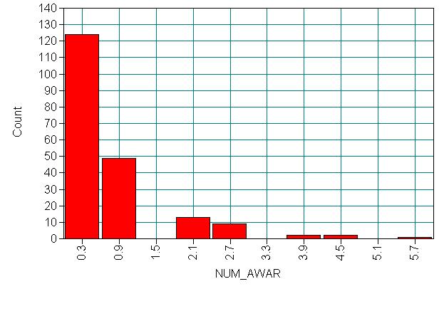
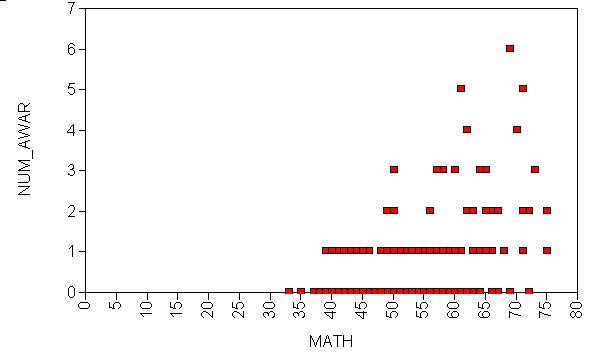
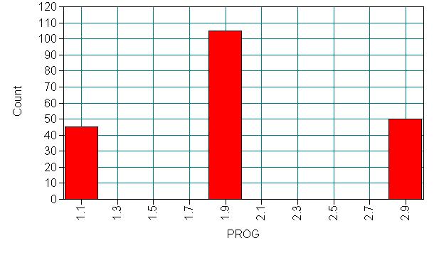
The data for this example were simulated and are in the file https://stats.idre.ucla.edu/wp-content/uploads/2016/02/poisson_sim.dat. In this example, num_awards is the outcome variable and indicates the number of awards earned by students at a single high school in a single year, math is a continuous predictor variable and represents students’ scores on their math final exam, and prog is a categorical predictor variable with three levels indicating the type of program in which the students were enrolled.
Let’s look at the data. It is always a good idea to start with descriptive statistics.
Data:
File is g:daehttps://stats.idre.ucla.edu/wp-content/uploads/2016/02/poisson_sim.dat;
Variable:
Names are
id num_awards prog math p1 p2 p3;
Missing are all (-9999);
usevariables are num_awards prog p1 p2 p3 math;
analysis:
type = basic;
plot: type is plot1;
RESULTS FOR BASIC ANALYSIS


     ESTIMATED SAMPLE STATISTICS


           Means
              NUM_AWAR      PROG          P1            P2            P3
              ________      ________      ________      ________      ________
      1         0.630         2.025         0.225         0.525         0.250


           Means
              MATH
              ________
      1        52.645


           Covariances
              NUM_AWAR      PROG          P1            P2            P3
              ________      ________      ________      ________      ________
 NUM_AWAR       1.103
 PROG          -0.001         0.474
 P1            -0.097        -0.231         0.174
 P2             0.194        -0.013        -0.118         0.249
 P3            -0.097         0.244        -0.056        -0.131         0.188
 MATH           4.879        -0.966        -0.590         2.146        -1.556


           Covariances
              MATH
              ________
 MATH          87.329


           Correlations
              NUM_AWAR      PROG          P1            P2            P3
              ________      ________      ________      ________      ________
 NUM_AWAR       1.000
 PROG          -0.001         1.000
 P1            -0.221        -0.802         1.000
 P2             0.370        -0.038        -0.566         1.000
 P3            -0.214         0.817        -0.311        -0.607         1.000
 MATH           0.497        -0.150        -0.151         0.460        -0.385


           Correlations
              MATH
              ________
 MATH           1.000


     MAXIMUM LOG-LIKELIHOOD VALUE FOR THE UNRESTRICTED (H1) MODEL IS     293.292
Analysis methods you might consider
Below is a list of some analysis methods you may have encountered. Some of the methods listed are quite reasonable, while others have either fallen out of favor or have limitations.
- Poisson regression – Poisson regression is often used for modeling count data. Poisson regression has a number of extensions useful for count models.
- Negative binomial regression – Negative binomial regression can be used for over-dispersed count data, that is when the conditional variance exceeds the conditional mean. It can be considered as a generalization of Poisson regression since it has the same mean structure as Poisson regression and it has an extra parameter to model the over-dispersion. If the conditional distribution of the outcome variable is over-dispersed, the confidence intervals for Negative binomial regression are likely to be narrower as compared to those from a Poisson regression.
- Zero-inflated regression model – Zero-inflated models attempt to account for excess zeros. In other words, two kinds of zeros are thought to exist in the data, "true zeros" and "excess zeros". Zero-inflated models estimate two equations simultaneously, one for the count model and one for the excess zeros.
- OLS regression – Count outcome variables are sometimes log-transformed and analyzed using OLS regression. Many issues arise with this approach, including loss of data due to undefined values generated by taking the log of zero (which is undefined) and biased estimates.
Poisson regression analysis
In the Mplus syntax below, we specify that the variables to be used in the Poisson regression are num_awards, p2, p3 and math. (The variables p2 and p3 are indicator variables for prog.) We also specify that num_awards is a count variable. (Because the variable name num_awards has more than eight characters, we get a warning in the output that this variable name has been truncated to eight characters.) By default, Mplus uses restricted maximum likelihood (MLR), so robust standard errors are given in the output. The MLR standard errors are computed using a sandwich estimator. These are what we generally call robust standard errors. Cameron and Trivedi (2009) recommend the use of robust standard errors when estimating a Poisson model. If you do not want robust standard errors, you can use the analysis: estimator = ml; block.
Data:
File is g:daehttps://stats.idre.ucla.edu/wp-content/uploads/2016/02/poisson_sim.dat;
Variable:
Names are
id num_awards prog math p1 p2 p3;
Missing are all (-9999) ;
usevariables are num_awards p2 p3 math;
count is num_awards;
model:
num_awards on p2 p3 math;
MODEL FIT INFORMATION

Number of Free Parameters                        4

Loglikelihood

          H0 Value                        -182.752
          H0 Scaling Correction Factor       0.976
            for MLR

Information Criteria

          Akaike (AIC)                     373.505
          Bayesian (BIC)                   386.698
          Sample-Size Adjusted BIC         374.025
            (n* = (n + 2) / 24)


MODEL RESULTS

                                                    Two-Tailed
                    Estimate       S.E.  Est./S.E.    P-Value

 NUM_AWARDS ON
    P2                 1.084      0.321      3.376      0.001
    P3                 0.370      0.400      0.924      0.356
    MATH               0.070      0.010      6.723      0.000

 Intercepts
    NUM_AWARDS        -5.247      0.646     -8.123      0.000
In the syntax below, some of the variables in the model are given labels. These labels must be in parentheses and must be the last item listed on the line, so the model is broken up over several lines. We have given the label a2 to the indicator variable p2, and the label a3 to the indicator variable p3. Once we have assigned labels to the variables, we can use those labels in the model test block. Setting both a2 and a3 to 0 allows us to get the two degree-of-freedom test of the variable prog.
Data:
File is g:daehttps://stats.idre.ucla.edu/wp-content/uploads/2016/02/poisson_sim.dat;
Variable:
Names are
id num_awards prog math p1 p2 p3;
Missing are all (-9999);
usevariables are num_awards p2 p3 math;
count is num_awards;
model:
num_awards on
p2 (a2)
p3 (a3)
math;
model test:
a2 = 0;
a3 = 0;
< - some output omitted - >MODEL FIT INFORMATION Number of Free Parameters 4 Loglikelihood H0 Value -182.752 H0 Scaling Correction Factor 0.976 for MLR Information Criteria Akaike (AIC) 373.505 Bayesian (BIC) 386.698 Sample-Size Adjusted BIC 374.025 (n* = (n + 2) / 24) Wald Test of Parameter Constraints Value 14.838 Degrees of Freedom 2 P-Value 0.0006
We can see that the variable prog, as a whole, is statistically significant. To help assess the fit of the model, we can look at the model fit statistics in the output. Several measures of goodness of fit are provided. For both the AIC and BIC, smaller is better.
To obtain the results as incident rate ratios, we need to use the model constraint block. Again, we use labels to refer to the variables in the model. In the model constraint block, we use the new statement to label the new parameters, which will be the exponentiated parameters from the model.
Data:
File is g:daehttps://stats.idre.ucla.edu/wp-content/uploads/2016/02/poisson_sim.dat;
Variable:
Names are
id num_awards prog math p1 p2 p3;
Missing are all (-9999);
usevariables are num_awards p2 p3 math;
count is num_awards;
model:
num_awards on
p2 (a2)
p3 (a3)
math (a1);
model constraint:
new(p2_exp p3_exp math_exp);
p2_exp = exp(a2);
p3_exp = exp(a3);
math_exp = exp(a1);
MODEL FIT INFORMATION Number of Free Parameters 4 Loglikelihood H0 Value -182.752 H0 Scaling Correction Factor 0.976 for MLR Information Criteria Akaike (AIC) 373.505 Bayesian (BIC) 386.698 Sample-Size Adjusted BIC 374.025 (n* = (n + 2) / 24) MODEL RESULTS Two-Tailed Estimate S.E. Est./S.E. P-Value NUM_AWARDS ON P2 1.084 0.321 3.376 0.001 P3 0.370 0.400 0.924 0.356 MATH 0.070 0.010 6.723 0.000 Intercepts NUM_AWARDS -5.247 0.646 -8.123 0.000 New/Additional Parameters P2_EXP 2.956 0.949 3.115 0.002 P3_EXP 1.447 0.580 2.497 0.013 MATH_EXP 1.073 0.011 95.830 0.000
Recall the form of our model equation:
log(num_awards) = Intercept + b1(prog=2) + b2(prog=3) + b3math.
This implies:
num_awards = exp(Intercept + b1(prog=2) + b2(prog=3)+ b3math) = exp(Intercept) * exp(b1(prog=2)) * exp(b2(prog=3)) * exp(b3math)
Things to consider
- When there seems to be an issue of dispersion, we should first check if our model is appropriately specified, such as omitted variables and functional forms. For example, if we omitted the predictor variable prog in the example above, our model would seem to have a problem with over-dispersion. In other words, a mis-specified model could present a symptom like an over-dispersion problem.
- Assuming that the model is correctly specified, you may want to test for over-dispersion. There are several tests of the alpha parameter, including the likelihood ratio test.
- One common cause of over-dispersion is excess zeros, which in turn are generated by an additional data generating process. In this situation, zero-inflated model should be considered.
- If the data generating process does not allow for any 0s (such as the number of days spent in the hospital), then a zero-truncated model may be more appropriate.
- Count data often have an exposure variable, which indicates the number of times the event could have happened. This variable should be incorporated into your Poisson model by taking the log of the exposure variable and constraining its estimate to 1.
- The outcome variable in a Poisson regression cannot have negative numbers, and the exposure cannot have 0s.
- The diagnostics for Poisson regression are different from those for OLS regression. The assumptions of the model should be checked (see Cameron and Trivedi (1998) and Dupont (2002) for more information).
- Poisson regression is estimated via maximum likelihood estimation. It usually requires a large sample size.
See also
References
- Cameron, A. C. and Trivedi, P. K. 2009. Microeconometrics Using Stata. College Station, TX: Stata Press.
- Cameron, A. C. and Trivedi, P. K. 1998. Regression Analysis of Count Data. New York: Cambridge Press.
- Cameron, A. C. Advances in Count Data Regression Talk for the Applied Statistics Workshop, March 28, 2009. http://cameron.econ.ucdavis.edu/racd/count.html .
- Dupont, W. D. 2002. Statistical Modeling for Biomedical Researchers: A Simple Introduction to the Analysis of Complex Data. New York: Cambridge Press.
- Long, J. S. 1997. Regression Models for Categorical and Limited Dependent Variables. Thousand Oaks, CA: Sage Publications.
- Long, J. S. and Freese, J. 2006. Regression Models for Categorical Dependent Variables Using Stata, Second Edition. College Station, TX: Stata Press.


