Note: This example was done using Mplus version 6.12. The syntax may not work, or may function differently, with other versions of Mplus.
The tobit model, also called a censored regression model, is designed to estimate linear relationships between variables when there is either left- or right-censoring in the dependent variable (also known as censoring from below and above, respectively). Censoring from above takes place when cases with a value at or above some threshold, all take on the value of that threshold, so that the true value might be equal to the threshold, but it might also be higher. In the case of censoring from below, values those that fall at or below some threshold are censored.
Please note: The purpose of this page is to show how to use various data analysis commands. It does not cover all aspects of the research process which researchers are expected to do. In particular, it does not cover data cleaning and checking, verification of assumptions, model diagnostics and potential follow-up analyses.
Examples of tobit analysis
Example 1.
In the 1980s there was a federal law restricting speedometer readings to no more than 85 mph. So if you wanted to try and predict a vehicle’s top-speed from a combination of horse-power and engine size, you would get a reading no higher than 85, regardless of how fast the vehicle was really traveling. This is a classic case of right-censoring (censoring from above) of the data. The only thing we are certain of is that those vehicles were traveling at least 85 mph.
Example 2. A research project is studying the level of lead in home drinking water as a function of the age of a house and family income. The water testing kit cannot detect lead concentrations below 5 parts per billion (ppb). The EPA considers levels above 15 ppb to be dangerous. These data are an example of left-censoring (censoring from below).
Example 3. Consider the situation in which we have a measure of academic aptitude (scaled 200-800) which we want to model using reading and math test scores, as well as, the type of program the student is enrolled in (academic, general, or vocational). The problem here is that students who answer all questions on the academic aptitude test correctly receive a score of 800, even though it is likely that these students are not “truly” equal in aptitude. The same is true of students who answer all of the questions incorrectly. All such students would have a score of 200, although they may not all be of equal aptitude.
Description of the data
Let’s pursue Example 3 from above.
We have a hypothetical data file, tobit.dta with 200 observations.
The academic aptitude variable is apt
Lets start by looking at some descriptive statistics generated in another package. The first table gives the descriptive statistics for the three continuous variables, and the second table tabulates the categorical variable prog. As expected the highest value of apt is 800. In this dataset, the lowest value of apt is 352 indicating that no students received a score of 200 (i.e., the lowest score possible), thus even though censoring from below was possible, it does not occur in this dataset.
    Variable |       Obs        Mean    Std. Dev.       Min        Max
-------------+--------------------------------------------------------
         apt |       200     640.035    99.21903        352        800
        read |       200       52.23    10.25294         28         76
        math |       200      52.645    9.368448         33         75


    type of |
    program |      Freq.     Percent        Cum.
------------+-----------------------------------
   academic |         45       22.50       22.50
    general |        105       52.50       75.00
 vocational |         50       25.00      100.00
------------+-----------------------------------
      Total |        200      100.00
As we mentioned above, even if you’ve already run descriptive statistics in another package, you probably want to run an Mplus model with type=basic to make sure your data has been read in properly. The input file for such a model is shown below. We have also used the type = plot1 option of the plot command, so that we can use Mplus to generate histograms and scatterplots.
Data:
  file is https://stats.idre.ucla.edu/wp-content/uploads/2016/02/tobit.dat;
Variable:
  names are id read math prog apt prog1 prog2 prog3;
  usevariables are read math apt prog1 prog2 prog3;
Analysis:
  type = basic;
Plot:
  type = plot1;
As we mentioned above, you will want to look at this output carefully to be sure that the dataset was read into Mplus correctly. For example, checking to make sure that you have the correct number of observations, and that the variables all have means that are close to those from the descriptive statistics generated in a general purpose statistical package. If there are missing values for some or all of the variables, the descriptive statistics generated by Mplus may not match those from a general purpose statistical package exactly, because by default, Mplus versions 5.0 and later use maximum likelihood based procedures for handling missing values. Looking at the output shown below we can confirm that the number of observations is correct and that the means of the variables are consistent with those from a general purpose statistical package. Later on we will use the variance of apt as a point of comparison, so we will make note of this variance (9795.194) shown on the diagonal of the covariance matrix below.
SUMMARY OF ANALYSIS

Number of groups                                                 1
Number of observations                                         200

<output omitted>

     ESTIMATED SAMPLE STATISTICS


           Means
              READ          MATH          APT           PROG1         PROG2
              ________      ________      ________      ________      ________
      1        52.230        52.645       640.035         0.225         0.525


           Means
              PROG3
              ________
      1         0.250


           Covariances
              READ          MATH          APT           PROG2         PROG3
              ________      ________      ________      ________      ________
 READ         105.123
 MATH          63.615        87.768
 APT          656.273       681.595      9844.416
 PROG2          2.075         2.157        19.906         0.251
 PROG3         -1.515        -1.564       -19.677        -0.132         0.188


           Correlations
              READ          MATH          APT           PROG2         PROG3
              ________      ________      ________      ________      ________
 READ           1.000
 MATH           0.662         1.000
 APT            0.645         0.733         1.000
 PROG2          0.404         0.460         0.401         1.000
 PROG3         -0.340        -0.385        -0.457        -0.607         1.000
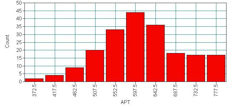
The plot command included in the input file above allows us to view histograms of our variables. We can view the histogram by clicking on the "Graph" menu, and then moving down to click on "View graphs." In the window that appears select "Histograms" and click "view." A second window will appear, where we can select the variable we wish to plot. Below is a histogram of apt.

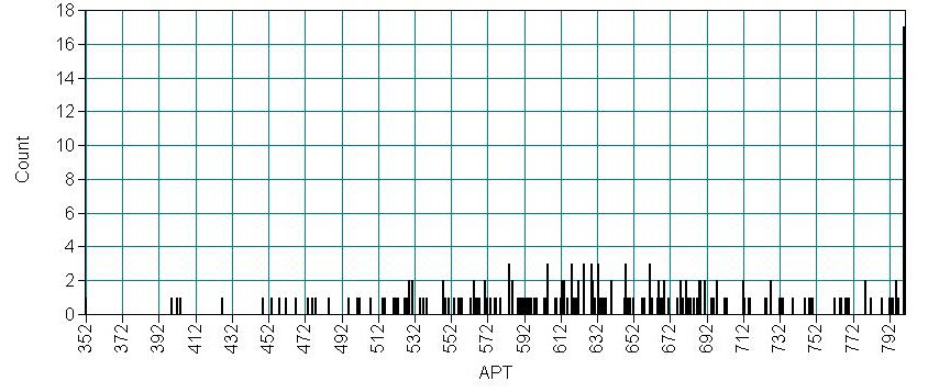
Looking at the above histogram showing the distribution of apt, we can see the censoring in the data, that is, there are more cases with scores of 750 to 800 (i.e., the bin labeled 777.5) than one would expect looking at the rest of the distribution. Below is an alternative histogram that further highlights the excess of cases where apt=800. To produce this graph we proceeded as before, but after we selected apt as the variable to be plotted, we moved to the "Display properties" tab (in the same window), here we set the number of bins to be the range of apt plus one (800-352+1=449), this produces a histogram with a bin for each integer value from 352 to 800. Because apt is continuous, most values of apt are unique in the dataset, although close to the center of the distribution there are a few values of apt that have two or three cases. The spike on the far right of the histogram is the bar for cases where apt=800, the height of this bar relative to all the others clearly shows the excess number of cases with this value.

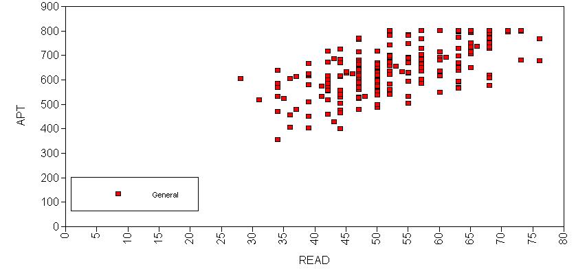
Next we’ll explore the bivariate relationships in our dataset. We can view the histogram by going to the "Graph" menu, and down to "View graphs," then selecting "Scatterplots" in the window that appears. Clicking view will show a second window, where we can select the variables we wish to plot. Below is a scatterplot showing read and apt. Note the collection of cases near the top of the scatterplot, due to the censoring in the distribution of apt.

Analysis methods you might consider
Below is a list of some analysis methods you may have encountered. Some of the methods listed are quite reasonable while others have either fallen out of favor or have limitations.
- Tobit regression, the focus of this page.
- OLS Regression – You could analyze these data using OLS regression. OLS regression will treat the 800 as the actual values and not as the lower limit of the top academic aptitude. A limitation of this approach is that when the variable is censored, OLS provides inconsistent estimates of the parameters, meaning that the coefficients from the analysis will not necessarily approach the "true" population parameters as the sample size increases. See Long (1997, chapter 7) for a more detailed discussion of problems of using OLS regression with censored data.
- Truncated Regression – There is sometimes confusion about the difference between truncated data and censored data. With censored variables, all of the observations are in the dataset, but we don’t know the "true" values of some of them. With truncation some of the observations are not included in the analysis because of the value of the variable. When a variable is censored, regression models for truncated data provide inconsistent estimates of the parameters. See Long (1997, chapter 7) for a more detailed discussion of problems of using regression models for truncated data to analyze censored data.
Tobit analysis
Below is the content of an Mplus input file for a tobit regression model. Because we are not using all of the variables in the dataset in the model, we use the usevariables option of the variables command to indicate which variables should be included in the model. The censored option declares that the variable apt is censored. The (a) following apt on the censored option indicates that the variable is censored from above (i.e., right censoring). If we had censoring from below (i.e., left-censoring), we would have used the (b) option instead. By default in version 6.12, Mplus uses a robust weighted least squares estimator. You can use maximum likelihood estimation with robust standard errors by specifying estimator = mlr in the analysis command. If you would like maximum likelihood estimation without robust standard errors, use estimator = ml in the analysis command.
data:
  file is https://stats.idre.ucla.edu/wp-content/uploads/2016/02/tobit.dat ;
variable:
  names are id read math prog apt prog1 prog2 prog3;
  usevariables are read math apt prog2 prog3;
  censored are apt (a);
model:
  apt on read math prog2 prog3;
output:
   stdyx;
SUMMARY OF ANALYSIS

Number of groups                                                 1
Number of observations                                         200

Number of dependent variables                                    1
Number of independent variables                                  4
Number of continuous latent variables                            0

Observed dependent variables

  Censored
   APT

Observed independent variables
   READ        MATH        PROG2       PROG3


Estimator                                                    WLSMV
Maximum number of iterations                                  1000
Convergence criterion                                    0.500D-04
Maximum number of steepest descent iterations                   20
Parameterization                                             DELTA
- At the top of the output we see that 200 observations were used.
- From the output we see that the model includes one censored dependent (i.e., outcome) variable and 4 independent (predictor) variables.
- The analysis summary is followed by a block of technical information about the model, which we will not discuss except to note that the estimator is listed as WLSMV (the default).
SUMMARY OF CENSORED LIMITS

      APT              800.000


THE MODEL ESTIMATION TERMINATED NORMALLY
- The section headed SUMMARY OF CENSORED LIMITS describes the censoring of values in the dataset, Mplus has correctly concluded that the maximum score for apt is 800.
MODEL FIT INFORMATION

Number of Free Parameters 6

Chi-Square Test of Model Fit

Value 0.000*
Degrees of Freedom 0
P-Value 0.0000

* The chi-square value for MLM, MLMV, MLR, ULSMV, WLSM and WLSMV cannot be used
for chi-square difference testing in the regular way. MLM, MLR and WLSM
chi-square difference testing is described on the Mplus website. MLMV, WLSMV,
and ULSMV difference testing is done using the DIFFTEST option.

RMSEA (Root Mean Square Error Of Approximation)

Estimate 0.000
90 Percent C.I. 0.000 0.000
Probability RMSEA <= .05 0.000

CFI/TLI

CFI 1.000
TLI 1.000

Chi-Square Test of Model Fit for the Baseline Model

Value 930585.250
Degrees of Freedom 5
P-Value 0.0000

WRMR (Weighted Root Mean Square Residual)

Value 0.000
MODEL RESULTS

                                                    Two-Tailed
                    Estimate       S.E.  Est./S.E.    P-Value

 APT      ON
    READ               2.698      0.637      4.234      0.000
    MATH               5.914      0.774      7.640      0.000
    PROG2            -12.715     13.525     -0.940      0.347
    PROG3            -46.144     14.233     -3.242      0.001

 Intercepts
    APT              209.568     33.189      6.314      0.000

 Residual Variances
    APT             4313.421    504.344      8.553      0.000
- The section titled MODEL RESULTS includes the coefficient estimates (labeled
Estimate), their standard errors, the ratio of each estimate to its standard
error (i.e., the z-score, labeled Est./S.E.), and the associated p-values.
The coefficients for read and math are statistically significant, as is the
coefficient for prog=3. Tobit regression coefficients are
interpreted in a similar manner to OLS regression coefficients; however, the linear effect
is on the uncensored latent variable, not the observed outcome. See McDonald and Moffitt (1980) for more details.
- For a one unit increase in read, there is a 2.7 point increase in the predicted value of apt.
- A one unit increase in math is associated with a 5.91 unit increase in the predicted value of apt.
- The residual variance of apt is 4313.42. Some packages give the square root of this parameter denoted sigma. This value can be compared to the variance of apt (9795.194 in the output from type=basic), a substantial reduction. Mplus also gives the standard error, est./s.e. and an associated p-value for the residual variance of apt. That the residual variance is statistically significant means that the estimated value (9795.194) is statistically significantly different from 0. The validity of this test is a matter of debate among statisticians, and some programs will produce the estimate and standard error, but not the test of statistical significance.
Because we used the stdyx option of the output command, the output includes standardized coefficients. We did this primarily to obtain the R-square values for the output variables, so we have omitted the standardized output to save space. Based on this output, the model explains about 62% of the variance in apt.
<output omitted>

R-SQUARE

    Observed                   Residual
    Variable        Estimate   Variance

    APT                0.616
We may also want to test that the coefficients for prog2, and prog3, all equal to zero. This type of test can also be described as an overall test for the effect of prog. There are multiple ways to test this type of hypothesis, the model test command requests one of them, a Wald test. The Mplus input file shown below is similar to the first regression model, except that the coefficients for prog2, and prog3 are assigned the names p2, and p3, respectively. Note that each variables to be tested must be alone on a line followed by its label in parentheses. In the model test command, these coefficient names (i.e., p2, and p3) are used to test that each of the coefficients is equal to 0.
Data:
  File is https://stats.idre.ucla.edu/wp-content/uploads/2016/02/tobit.dat;
Variable:
  Names are id read math prog apt prog1 prog2 prog3;
  usevariables are read math apt prog2 prog3;
  censored are apt (a);
Model:
  apt on read math
    prog2 (p1)
    prog3 (p2);
Model test:
  p1 = 0;
  p2 = 0;
The majority of the output from this model is the same as the first model, so we will only show part of the output generated by the model test command.
Wald Test of Parameter Constraints

          Value                             11.906
          Degrees of Freedom                     2
          P-Value                           0.0026
The test statistic of 11.906, with 2 degrees of freedom and an associated p-value of 0.0026 indicates that the overall effect of prog is statistically significant.
We can also test additional hypotheses about the differences in the coefficients for different levels of prog. Below we test that the coefficient for prog2 is equal to the coefficient for prog3. In the output below we see that the two coefficient are significantly different.
Data:
  File is https://stats.idre.ucla.edu/wp-content/uploads/2016/02/tobit.dat;
Variable:
  Names are id read math prog apt prog1 prog2 prog3;
    Missing are all (-9999) ;
    usevariables are read math apt prog2 prog3;
    censored are apt (a);
Model:
  apt on read math
    prog2 (p1)
    prog3 (p2);
Model test:
  p1 = p2;


Wald Test of Parameter Constraints

          Value                              6.979
          Degrees of Freedom                     1
          P-Value                           0.0082
The test statistic of 6.979, with 1 degree of freedom and an associated p-value of 0.0082 indicates that the coefficient for prog=2 is significantly different from the coefficient for prog=3.
See also
References
Long, J. S. 1997. Regression Models for Categorical and Limited Dependent Variables. Thousand Oaks, CA: Sage Publications.
McDonald, J. F. and Moffitt, R. A. 1980. The Uses of Tobit Analysis. The Review of Economics and Statistics Vol 62(2): 318-321.
Tobin, J. 1958. Estimation of relationships for limited dependent variables. Econometrica 26: 24-36.
