Mplus Textbook
Examples
Solving Examples from EQS Manual Using Mplus
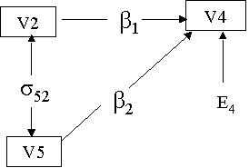
Example 1: A Simple Regression Model on page 15
The data file manul1.txt is the covariance matrix and can be downloaded here.
Title: Mplus code for example 1 from EQS manual on page 15
Data: File is https://stats.idre.ucla.edu/wp-content/uploads/2016/02/manul1.txt;
      Type is covariance ;
      Nobservations = 932;
Variable: Names are y1 y2 y3 y4 y5 y6;
          usevariables are y2 y4 y5;
Analysis: Type is general;
          estimator is gls;
Model: y4 on y2 y5; !! Setting up the regression model;
       y2 y5;       !! Variance of y2 and y5 are free parameters to be
                    !! estimated;
MODEL RESULTS
Estimates S.E. Est./S.E.
 Y4       ON
    Y2                 0.457    0.031     14.724
    Y5                -0.192    0.031     -6.272
 Y5       WITH
    Y2                -3.889    0.336    -11.574
 Variances
    Y2                 9.364    0.434     21.576
    Y5                 9.610    0.445     21.575
 Residual Variances
    Y4                 6.991    0.324     21.575
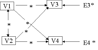
Example 2: A Two-Equation Path Model on page 22
The data file https://stats.idre.ucla.edu/wp-content/uploads/2016/02/manul1.txt used is the same as in previous example.
Title: Mplus code A Two-Equation Path Model on page 22
Data: File is https://stats.idre.ucla.edu/wp-content/uploads/2016/02/manul1.txt;
      Type is covariance ;
      Nobservations = 932;
Variable: Names are y1 y2 y3 y4 y5 y6;
          usevariables are y1 y2 y3 y4;
Analysis: Type is general;
          estimator is ml;
Model: y3 on y1 y2;
       y4 on y1 y2;
       y1 y2;
       y1 with y2;
MODEL RESULTS
Estimates S.E. Est./S.E.
 Y3       ON
    Y1                 0.455    0.037     12.413
    Y2                 0.206    0.041      4.991
 Y4       ON
    Y1                 0.158    0.034      4.660
    Y2                 0.420    0.038     11.048
 Y1       WITH
    Y2                 6.939    0.413     16.815
 Y4       WITH
    Y3                 4.277    0.289     14.802
 Variances
    Y1                11.821    0.548     21.587
    Y2                 9.354    0.433     21.587
 Residual Variances
    Y3                 8.370    0.388     21.587
    Y4                 7.113    0.329     21.587
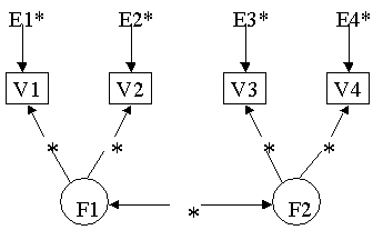
Example 3: A Factor Analysis Model on page 29
The data file https://stats.idre.ucla.edu/wp-content/uploads/2016/02/manul1.txt used is the same as in previous example.
Title: Mplus code: A Factor Analysis Model on page 29
Data: File is https://stats.idre.ucla.edu/wp-content/uploads/2016/02/manul1.txt;
      Type is covariance ;
      Nobservations = 932;
Variable: Names are y1 y2 y3 y4 y5 y6;
          usevariables are y1 y2 y3 y4;
Analysis: Type = general;
          estimator is gls;
Model: f1 by y1* (1)
             y2  (2);
       f2 by y3* (1)
             y4  (2);
       f1@1 f2@1;
       y1 y3 (3);  !! setting the residual variance of
       y2 y4 (4);  !! y1 and y3 to be equal.
       y1 with y3 (5); !! setting the residual covariance
       y2 with y4 (5); !! of (y1, y3) equal to (y2, y4).
       f1 with f2;
MODEL RESULTS
Estimates S.E. Est./S.E.
 F1       BY
    Y1                 2.937    0.090     32.816
    Y2                 2.446    0.081     30.261
 F2       BY
    Y3                 2.937    0.090     32.816
    Y4                 2.446    0.081     30.261
 F1       WITH
    F2                 0.685    0.026     26.574
 Y1       WITH
    Y3                 0.901    0.122      7.415
 Y2       WITH
    Y4                 0.901    0.122      7.415
 Variances
    F1                 1.000    0.000      0.000
    F2                 1.000    0.000      0.000
 Residual Variances
    Y1                 3.519    0.267     13.176
    Y2                 3.644    0.206     17.717
    Y3                 3.519    0.267     13.176
    Y4                 3.644    0.206     17.717
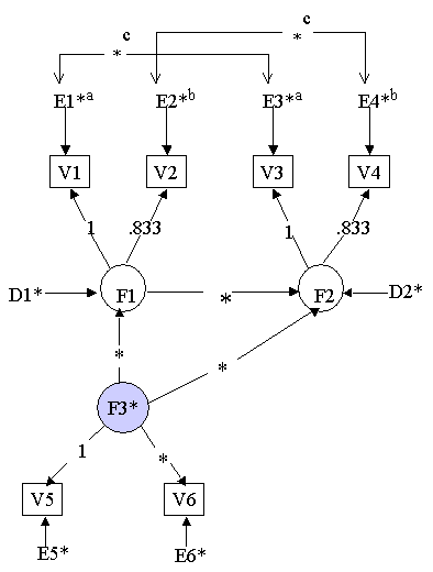
Example 4: A Complete Latent Variable Model on page 33
The data file https://stats.idre.ucla.edu/wp-content/uploads/2016/02/manul1.txt used is the same as in previous example.
Title: Mplus code:  A COMPLETE LATENT VARIABLE MODEL
       (EXAMPLE IN EQS MANUAL P.33)
Data: File is https://stats.idre.ucla.edu/wp-content/uploads/2016/02/manul1.txt;
      Type is covariance ;
      Nobservations = 932;
Variable: Names are y1 y2 y3 y4 y5 y6;
          Usevariables are y1 y2 y3 y4 y5 y6;

Analysis: Type = general;
          estimator is ml;
Model: f1 by y1 y2@.833;
       f2 by y3 y4@.833;
       f3 by y5 y6;
       f1 on f3;
       f2 on f1 f3;
       y1 y3 (3);  !! setting the residual variance of
       y2 y4 (4);  !! y1 and y3 to be equal.
       y1 with y3 (5); !! setting the residual covariance
       y2 with y4 (5); !! of (y1, y3) equal to (y2, y4).
TESTS OF MODEL FIT
Chi-Square Test of Model Fit
          Value                             13.491
          Degrees of Freedom                     9
          P-Value                           0.1416
Chi-Square Test of Model Fit for the Baseline Model
          Value                           2133.653
          Degrees of Freedom                    15
          P-Value                           0.0000
CFI/TLI
          CFI                                0.998
          TLI                                0.996
Loglikelihood
          H0 Value                      -13071.689
          H1 Value                      -13064.944
Information Criteria
          Number of Free Parameters             12
          Akaike (AIC)                   26167.379
          Bayesian (BIC)                 26225.427
          Sample-Size Adjusted BIC       26187.316
            (n* = (n + 2) / 24)
RMSEA (Root Mean Square Error Of Approximation)
          Estimate                           0.023
          90 Percent C.I.                    0.000  0.047
          Probability RMSEA <= .05           0.971
SRMR (Standardized Root Mean Square Residual)
Value 0.015
MODEL RESULTS
Estimates S.E. Est./S.E.
 F1       BY
    Y1                 1.000    0.000      0.000
    Y2                 0.833    0.000      0.000
 F2       BY
    Y3                 1.000    0.000      0.000
    Y4                 0.833    0.000      0.000
 F3       BY
    Y5                 1.000    0.000      0.000
    Y6                 0.537    0.043     12.385
 F1       ON
    F3                -0.630    0.056    -11.186
 F2       ON
    F1                 0.593    0.047     12.685
    F3                -0.241    0.055     -4.393
 Y1       WITH
    Y3                 0.905    0.121      7.449
 Y2       WITH
    Y4                 0.905    0.121      7.449
 Variances
    F3                 6.609    0.638     10.357
 Residual Variances
    Y1                 3.604    0.201     17.967
    Y2                 3.591    0.164     21.867
    Y3                 3.604    0.201     17.967
    Y4                 3.591    0.164     21.867
    Y5                 2.991    0.498      6.007
    Y6                 2.593    0.183     14.183
    F1                 5.664    0.422     13.413
    F2                 4.510    0.335     13.471
Example 5: A Second-order Factor Analysis Model on page 38
The data file https://stats.idre.ucla.edu/wp-content/uploads/2016/02/manul1.txt used is the same as in previous example.
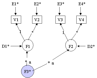
Title: Mplus code:  A SECOND-ORDER FACTOR ANALYSIS MODEL
       (EXAMPLE IN EQS MANUAL P.38)
Data: File is https://stats.idre.ucla.edu/wp-content/uploads/2016/02/manul1.txt;
      Type is covariance ;
      Nobservations = 932;
Variable: Names are y1 y2 y3 y4 y5 y6;
          usevariables are y1 y2 y3 y4 ;
Analysis: Type = general;
          estimator is gls;
Model: f1 by y1 y2;
       f2 by y3 y4;
       f3 by f1@0 f1 f2 (1);
       f3@1;
TESTS OF MODEL FIT
Chi-Square Test of Model Fit
          Value                             55.612
          Degrees of Freedom                     1
          P-Value                           0.0000
Chi-Square Test of Model Fit for the Baseline Model
          Value                            544.805
          Degrees of Freedom                     6
          P-Value                           0.0000
CFI/TLI
          CFI                                0.899
          TLI                                0.392
RMSEA (Root Mean Square Error Of Approximation)
          Estimate                           0.242
          90 Percent C.I.                    0.190  0.298
          Probability RMSEA <= .05           0.000
SRMR (Standardized Root Mean Square Residual)
Value 0.032
MODEL RESULTS
Estimates S.E. Est./S.E.
 F1       BY
    Y1                 1.000    0.000      0.000
    Y2                 0.847    0.042     20.158
 F2       BY
    Y3                 1.000    0.000      0.000
    Y4                 0.815    0.040     20.343
 F3       BY
    F1                 2.544    0.089     28.446
    F1                 2.544    0.089     28.446
    F2                 2.544    0.089     28.446
 Variances
    F3                 1.000    0.000      0.000
 Residual Variances
    Y1                 3.199    0.375      8.540
    Y2                 3.063    0.287     10.678
    Y3                 2.940    0.403      7.302
    Y4                 3.413    0.301     11.331
    F1                 1.976    0.438      4.514
    F2                 2.975    0.491      6.055
Example 6: A Nonstandard Model on page 104
The data file is https://stats.idre.ucla.edu/wp-content/uploads/2016/02/bag.txt.
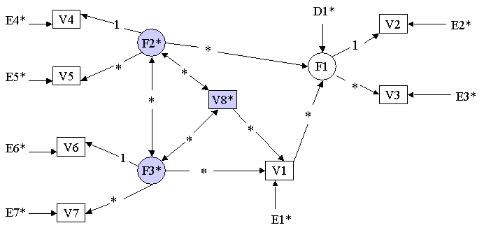
Title: Mplus code: Example 6: A Nonstandard Model on page 104
Data: File is https://stats.idre.ucla.edu/wp-content/uploads/2016/02/bag.txt;
      Type is correlation means stdeviations;
      Nobservations = 122;
Variable: Names are y1 y2 y3 y4 y5 y6 y7 y8;
          usevariables are y1 y2 y3 y4 y5 y6 y7 y8;
Analysis: Type = meanstructure;
          estimator is ml;
Model: f1 by y2 y3*1;
       f2 by y4 y5*1;
       f3 by y6 y7*1;
       y1 on f3 y8;
       f1 on f2 y1;
       f2 with f3;
       y8 with f2;
       y8 with f3;
MODEL RESULTS
Estimates S.E. Est./S.E.
 F1       BY
    Y2                 1.000    0.000      0.000
    Y3                 0.763    0.131      5.807
 F2       BY
    Y4                 1.000    0.000      0.000
    Y5                 1.234    0.398      3.096
 F3       BY
    Y6                 1.000    0.000      0.000
    Y7                 0.874    0.142      6.173
 F1       ON
    F2                 0.886    0.370      2.394
 F1       ON
    Y1                 0.557    0.138      4.027
 Y1       ON
    F3                 0.823    0.147      5.613
 Y1       ON
    Y8                -0.082    0.046     -1.761
 F2       WITH
    F3                 0.692    0.299      2.314
 Y8       WITH
    F2                -1.412    0.569     -2.481
    F3                -1.970    0.684     -2.878
 Means
    Y8                 0.000    0.329      0.000
 Intercepts
    Y1                 0.000    0.181      0.000
    Y2                 0.000    0.282      0.000
    Y3                 0.000    0.234      0.000
    Y4                 0.000    0.176      0.000
    Y5                 0.000    0.188      0.000
    Y6                 0.000    0.195      0.000
    Y7                 0.000    0.186      0.000
 Variances
    Y8                13.213    1.692      7.810
    F2                 1.234    0.528      2.338
    F3                 2.772    0.657      4.219
 Residual Variances
    Y1                 2.099    0.377      5.570
    Y2                 3.815    1.285      2.968
    Y3                 3.257    0.808      4.030
    Y4                 2.537    0.506      5.011
    Y5                 2.413    0.660      3.655
    Y6                 1.855    0.440      4.216
    Y7                 2.091    0.391      5.351
    F1                 4.902    1.365      3.591
Example 7: A Simulated Confirmatory Factory Analysis Example on page 117
The data file used is https://stats.idre.ucla.edu/wp-content/uploads/2016/02/data67.txt.
Title: Mplus code:
       A Simulated Confirmatory Factory Analysis Example on page 117
Data: https://stats.idre.ucla.edu/wp-content/uploads/2016/02/data67.txt;
Variable: Names are y1 y2 y3 y4 y5 y6 ;
          usevariables are y1 y2 y3 y4 y5 y6;
Analysis: Type = general;
          estimator is ml;
Model: f1 by y1* y2 y3;
       f2 by y4* y5 y6;
       f1 with f2;
       f1@1 f2@1;
MODEL RESULTS
Estimates S.E. Est./S.E.
 F1       BY
    Y1                 1.541    0.348      4.430
    Y2                 0.481    0.164      2.929
    Y3                 0.186    0.181      1.028
 F2       BY
    Y4                 0.663    0.154      4.294
    Y5                 0.871    0.162      5.364
    Y6                 0.180    0.140      1.284
 F1       WITH
    F2                 0.638    0.169      3.768
 Variances
    F1                 1.000    0.000      0.000
    F2                 1.000    0.000      0.000
 Residual Variances
    Y1                 0.414    0.923      0.448
    Y2                 0.789    0.182      4.338
    Y3                 1.369    0.275      4.977
    Y4                 0.590    0.165      3.567
    Y5                 0.292    0.207      1.413
    Y6                 0.761    0.154      4.944
Example 8: 2 GROUP EXAMPLE FROM WERTS ET AL 1976 on page 158
The data file used for this example is https://stats.idre.ucla.edu/wp-content/uploads/2016/02/page158.txt.
Title: Mplus code: EXAMPLE IN EQS MANUAL P. 158
Data: File is https://stats.idre.ucla.edu/wp-content/uploads/2016/02/page158.txt;
      Type is covariance ;
      Nobservations = 865 900;
      Ngroups = 2;
Variable: Names are y1 y2 y3 y4 ;
          usevariables are y1 y2 y3 y4;
Analysis: Type = general;
          estimator is ml;
Model: f1 by y1* y2;
       f2 by y3* y4;
       f1@1 f2@1;
       f1 with f2 (1);
Model g2: f1 with f2 (1);
TESTS OF MODEL FIT
Chi-Square Test of Model Fit
          Value                             10.884
          Degrees of Freedom                     7
          P-Value                           0.1436
Chi-Square Test of Model Fit for the Baseline Model
          Value                           5478.850
          Degrees of Freedom                    12
          P-Value                           0.0000
CFI/TLI
          CFI                                0.999
          TLI                                0.999
Loglikelihood
          H0 Value                      -21859.201
          H1 Value                      -21853.759
Information Criteria
          Number of Free Parameters             13
          Akaike (AIC)                   43744.403
          Bayesian (BIC)                 43815.590
          Sample-Size Adjusted BIC       43774.290
            (n* = (n + 2) / 24)
RMSEA (Root Mean Square Error Of Approximation)
          Estimate                           0.025
          90 Percent C.I.                    0.000  0.052
SRMR (Standardized Root Mean Square Residual)
Value 0.021
MODEL RESULTS
Estimates S.E. Est./S.E. Std StdYX
Group G1
 F1       BY
    Y1                 7.438    0.155     47.881    7.438    0.938
    Y2                 9.676    0.199     48.623    9.676    0.909
 F2       BY
    Y3                 7.283    0.152     48.003    7.283    0.920
    Y4                 5.192    0.114     45.507    5.192    0.902
 F1       WITH
    F2                 0.767    0.012     62.183    0.767    0.767
 Variances
    F1                 1.000    0.000      0.000    1.000    1.000
    F2                 1.000    0.000      0.000    1.000    1.000
 Residual Variances
    Y1                 7.590    1.023      7.418    7.590    0.121
    Y2                19.717    1.883     10.469   19.717    0.174
    Y3                 9.570    1.097      8.722    9.570    0.153
    Y4                 6.184    0.589     10.495    6.184    0.187
Group G2
 F1       BY
    Y1                 7.438    0.155     47.881    7.438    0.897
    Y2                 9.676    0.199     48.623    9.676    0.944
 F2       BY
    Y3                 7.283    0.152     48.003    7.283    0.931
    Y4                 5.192    0.114     45.507    5.192    0.884
 F1       WITH
    F2                 0.767    0.012     62.183    0.767    0.767
 Variances
    F1                 1.000    0.000      0.000    1.000    1.000
    F2                 1.000    0.000      0.000    1.000    1.000
 Residual Variances
    Y1                13.492    1.154     11.689   13.492    0.196
    Y2                11.466    1.702      6.735   11.466    0.109
    Y3                 8.181    1.065      7.678    8.181    0.134
    Y4                 7.513    0.621     12.090    7.513    0.218
R-SQUARE
Group G1
    Observed
    Variable  R-Square
    Y1           0.879
    Y2           0.826
    Y3           0.847
    Y4           0.813
Group G2
    Observed
    Variable  R-Square
    Y1           0.804
    Y2           0.891
    Y3           0.866
    Y4           0.782
Example 9: Growth in Wisc Scores on page 175
The data file used for this example is https://stats.idre.ucla.edu/wp-content/uploads/2016/02/manual9.txt.
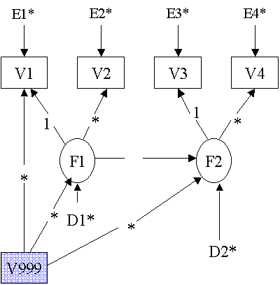
Example 10: Multiple Groups and Structured Means on page 186
The data file used for this example is https://stats.idre.ucla.edu/wp-content/uploads/2016/02/page186.txt.

