This seminar is a continuation of our Introduction to Mplus seminar. We will review the basics of Mplus syntax and show some examples for simple analyses, such as regression models for continuous and binary variables. Then we’ll move on to more advanced models, such as factor analysis, path analysis, growth curve models and latent class models. Some of the examples will be demonstrated by running Mplus in real time. The data files and the input files are zipped for an easy download and can be accessed by following the link.
Introduction
“We started to develop Mplus eleven years ago with the goal of providing applied researchers with powerful new statistical modeling techniques. We saw a wide gap between new statistical methods presented in the statistical literature and the statistical methods used by researchers in applied papers. Our goal was to help bridge this gap with easy-to-use but powerful software.” — February 2006, Preface to the Mplus User’s Guide.
Mplus has been very successful in achieving their goal and has been improving constantly ever since it was first released in 1998. Its general framework of continuous and categorical latent variables gives us a new framework to formulate statistical models. For example, not only we can perform growth curve analysis, but also latent class growth analysis; not only we can do discrete-time survival analysis, but also discrete-time survival mixture analysis. The possibilities of different ways of modeling make Mplus a very attractive piece of software. It offers several options to deal with the missing data issue, including maximum likelihood estimation and estimation based on the multiple imputed data sets.
Over the years, we have recommended to our clients the “get in and get out” approach with Mplus (and some other statistical packages) and it seems to us that this approach has worked well. This approach consists of a few steps: deciding the appropriate models for the study; deciding if switching to Mplus is necessary; preparing the data structure for Mplus using a familiar software package; and moving to Mplus and performing the analyses.
Our goal for this seminar is to help the transition process to Mplus. We will discuss the overall structure and syntax of Mplus input files. We will also discuss the usage of the Mplus 4 User’s Guide and the online resources for Mplus. Starting with some basic models, we will transit to some more advanced models.
Overall structure of Mplus input file
An input file defines the data set to use and the model to run. It is similar to a SAS program file, an SPSS syntax file and a Stata .do file. Below is an example of an input file. It is here to show the general structure of an input file. We are not going to explain what analysis it does.
Data:
      File is d:workdatarawtable3_4.dat ;
    Variable:
      names are a b c d freq;
      missing are all (-9999) ;
      usevariables are a b c d;
      weight is freq ; !default is frequency weight
      categorical are a b c d;
      classes = cl(2);
    Analysis:
      Type = mixture ;
      starts = 0;
    Model:
       %overall%
       [a$1*10 b$1*10 c$1*10 d$1*10] (1);
       %cl#1%
       [a$1*-10 b$1*-10 c$1*-10 d$1*-10] (2);
   plot:
      type= plot3;
      series is a(1) b(2) c(3) d(4);
Here are some characteristics of an input file:
- an input line can not exceed 80 characters in width;
- variable names can not exceed 8 characters in length;
- only one model per input file;
- only one output file per input file;
- comments start with “!”;
- the default of the analysis type is type = general;
- the keywords categorical and count are for outcome variables only;
- new variables can be defined using the” define” command.
Here are some characteristics of a data file:
- must be in ASCII format;
- can be in fixed format or delimited;
- can be raw data or correlation data;
- no variable names in the first line;
- only numeric variables are allowed;
- use stata2mplus to convert a Stata data file to an ASCII data file and an Mplus input file.
Overall review of Mplus syntax for the model command
Mplus has made a great effort to make the syntax as simple as possible. Since there are so many analyses that Mplus can perform, the model command can still get really involved. We have compiled a short list here for commonly used keywords.
- “on” for regression (regress response variable “on” predictor variables);
- “by” for factors (measured “by” observed variables);
- “with” for covariance (correlated “with”);
- “[x]” for means or intercepts;
- “x” alone means the variance of x;
- “*” for starting values;
- “@” for fixed values;
- “|” for random effects;
- use (_number_) to constrain a set of parameters to be equal.
Use of User’s Guide and online resources
The Mplus User’s Guide is an excellent reference both for Mplus syntax and for types of models possible in Mplus. It has the flavor of learning by doing. Its organization is very different from other user guides, such as that of Stata, SAS or SPSS. Examples for basic models can be found in the first chapter, and more advanced models are divided into later chapters. The section on syntax is near the end. A very important feature is that almost all of the examples in the Guide are included with the software itself. If one sees an interesting example, one can always run the model to see the output and to modify the example to suit one’s own modeling need. An equally important feature is that each example in the book has a counterpart of Monte Carlo simulation. In fact, the Monte Carlo simulation has been used for generating most of the data sets used in the User’s Guide. The help system of Mplus has A SUMMARY OF THE Mplus LANGUAGE for a quick reference.
The Mplus website has tremendous resources, with a very active discussion group on many topics for serious modelers and the website has many examples one can download. One can get access to the entire User’s Guide in PDF format from Mplus’ website. One can search the entire Mplus User’s Guide for examples and commands. It is a great place to learn new modeling possibilities and to learn Mplus language as well.
Post estimation
Mplus has three commands for post estimation. The output command, the savedata command and the plot command. The output command is used for requesting types of output to be included in the output file. For example, we can request sample statistics to be displayed by using the option sampstat in the output command. The savedata command is used for creating an ASCII data file for further data analysis. The plot command is needed for requesting plots. Mplus offers many model related plots and the controls over the plots are easy to use.
Simple examples
We will review how some simple models are done in Mplus. We will start with linear regression and then discuss models with binary outcomes.
Example 1. Where is the output for intercept? (linear regression)
The code below is for a simple linear regression with the dependent variable write regressed on the predictor variables female and read. So we use the keyword on in the model statement.
  Data:
    File is hsb2.dat ;
  Variable:
    Names are
       id female race ses schtyp prog read write math science socst;
    Missing are all (-9999) ;
    usevariables are female write read;
  Model:
    write on female read;

MODEL RESULTS
Estimates S.E. Est./S.E.
 WRITE    ON
    FEMALE             5.487    1.007      5.451
    READ               0.566    0.049     11.546
 Residual Variances
    WRITE             50.113    5.011     10.000
Notice that something is missing in the output. Yes, the intercept is missing. What does it mean? Be default, Mplus performs an analysis of covariance. To understand what it is doing, let’s perform this analysis manually in the fashion of covariance analysis. We create the covariance matrix for the variables write, female and read, and use this covariance matrix as the input for our analysis.
  Title: example of using covariance matrix.
         input data is an matrix:
         89.8436
         1.21369  .249221
         57.9967 -.271709  105.123;
  Data: file is cov.dat;
        type is covariance;
        nobservations = 200;
  Variable: names are write female read;
  Model: write on female read;

                   Estimates     S.E.  Est./S.E.

 WRITE    ON
    FEMALE             5.487    1.007      5.451
    READ               0.566    0.049     11.546

 Residual Variances
    WRITE             50.113    5.011     10.000
That shows that the analysis we did at the beginning of this example is just an analysis of covariance. In order to estimate the intercept, which is the expected mean holding values of predictor variables at zero, we need to tell Mplus that we are also interested in the analysis of means. This can be done easily by adding type = meanstructure to the analysis command. Every model has an analysis command associated with it. In this example, we don’t see the analysis command because we are using the default setting. The default setting is analysis: type = general. Models that can be estimated using type=general include regression analysis, path analysis, confirmatory factor analysis, structural equation modeling and growth curve modeling. Within any specific analysis setting, we can add more options, such as type = missing when the data set has missing values, and we don’t want to do listwise deletion. Or we can add type =meanstructure to have the mean or intercept displayed in the output window as we are going to do here.
  Data:
    File is hsb2.dat ;
  Variable:
    Names are
       id female race ses schtyp prog read write math science socst;
    Missing are all (-9999) ;
    usevariables are female write read;
  Analysis:
    type=meanstructure;
  Model:
    write on female read;
Estimates S.E. Est./S.E.
 WRITE    ON
    FEMALE             5.487    1.007      5.451
    READ               0.566    0.049     11.546
 Intercepts
    WRITE             20.228    2.693      7.511
 Residual Variances
    WRITE             50.113    5.011     10.000
Example 2. Is it a probit or a logit regression? (binary outcome)
Now let’s switch to binary outcomes. Using the same data set as in previous example, we create a new dichotomous variable called hon based on the variable write. We also declare that the new variable hon is a categorical variable. As we have mentioned before, the keyword categorical is for outcome variables only. If we have categorical variables as predictors, we have to make sure the dummy variables have been created for them (usually in another software package before the data are moved into Mplus).
  Data:
    File is hsb2.dat ;
  Variable:
    Names are
       id female race ses schtyp prog read write math science socst;
    Missing are all (-9999) ;
    usevariables are female math read hon;
    categorical is hon;
    define: hon = (write>60);
  Model:
    hon on female math read;
Observed dependent variables
  Binary and ordered categorical (ordinal)
   HON
Observed independent variables
   FEMALE      MATH        READ
Estimator                                                    WLSMV
Maximum number of iterations                                  1000
Convergence criterion                                    0.500D-04
Maximum number of steepest descent iterations                   20
Parameterization                                             DELTA
Input data file(s)
  hsb2.dat
Input data format FREE
SUMMARY OF CATEGORICAL DATA PROPORTIONS
    HON
      Category 1    0.755
      Category 2    0.245
(output omitted...)

MODEL RESULTS
Estimates S.E. Est./S.E.
 HON      ON
    FEMALE             0.574    0.246      2.335
    MATH               0.069    0.016      4.324
    READ               0.038    0.017      2.275
R-SQUARE
    Observed  Residual
    Variable  Variance  R-Square
HON 1.000 0.489
Now, is this a probit model or a logit model? Mplus is not very explicit about it. By default, it is a probit model. In case we don’t know the default, we can still tell that this is a probit model since it has an output section on R-square with residual variance of 1. This is what probit models assume. It assumes that the residual variance follows the standard normal distribution. Now did we miss something again? Yes. We don’t see the intercept. This is the exact same situation as we had with the linear regression. Adding type=meanstructure will give us the intercept, which Mplus calls “threshold”.
  Data:
    File is hsb2.dat ;
  Variable:
    Names are id female race ses schtyp prog
              read write math science socst;
    Missing are all (-9999) ;
    Usevariables are female math read hon;
    Categorical is hon;
    Define: hon = (write>60);
  Analysis: type=meanstructure;
  Model:
      hon on female math read;

MODEL RESULTS

                   Estimates     S.E.  Est./S.E.

 HON      ON
    FEMALE             0.574    0.246      2.335
    MATH               0.069    0.016      4.324
    READ               0.038    0.017      2.275

 Thresholds
    HON$1              6.887    1.063      6.482

R-SQUARE

    Observed  Residual
    Variable  Variance  R-Square

    HON          1.000     0.489
What about a logistic regression with the same data? To do a logistic regression, we will change the estimation method from the default method of WLSMV to ML.
  Data:
    File is hsb2.dat ;
  Variable:
    Names are id female race ses schtyp prog
              read write math science socst;
    Missing are all (-9999) ;
    Usevariables are female math read hon;
    Categorical is hon;
    Define: hon = (write>60);
  Analysis: estimator = ml;
  Model:
    hon on female math read;
Estimator                                                       ML
(output omitted...)
Link                                                         LOGIT
Cholesky                                                       OFF
Input data file(s)
  hsb2.dat
Input data format  FREE
SUMMARY OF CATEGORICAL DATA PROPORTIONS
    HON
      Category 1    0.755
      Category 2    0.245
THE MODEL ESTIMATION TERMINATED NORMALLY
TESTS OF MODEL FIT
Loglikelihood
H0 Value -78.085
Information Criteria
          Number of Free Parameters              4
          Akaike (AIC)                     164.170
          Bayesian (BIC)                   177.363
          Sample-Size Adjusted BIC         164.690
            (n* = (n + 2) / 24)
MODEL RESULTS
Estimates S.E. Est./S.E.
 HON        ON
    FEMALE             0.980    0.422      2.324
    MATH               0.123    0.031      3.931
    READ               0.059    0.027      2.224
 Thresholds
    HON$1             11.770    1.711      6.880
LOGISTIC REGRESSION ODDS RATIO RESULTS
 HON        ON
    FEMALE             2.664
    MATH               1.131
    READ               1.061
Advanced examples
Example 1. Exploratory factor analysis
Exploratory factor analysis has often been used to explore the variable structures. But most statistical software lacks the sophisticated techniques to deal with the missing value issue or binary variables. On the other hand, Mplus allows us to take care of both issues. Let’s start with a simple exploratory factor analysis. This example is taken from our Annotated SPSS Output Factor Analysis page. The data set has many variables, and we are only going to use item13 – item24, as they are all about instructors.
  Data:
    File is factor.dat ;
  Variable:
    Names are
       facsex facethn facnat facrank employm salary yrsteach yrsut degree
       sample remind nstud studrank studsex grade gpa satisfy religion psd
       item13 item14 item15 item16 item17 item18 item19 item20 item21 item22
       item23 item24 item25 item26 item27 item28 item29 item30 item31 item32
       item33 item34 item35 item36 item37 item38 item39 item40 item41 item42
       item43 item44 item45 item46 item47 item48 item49 item50 item51 item52
       race sexism racism rpolicy casteman competen sensitiv cstatus;
    Missing are all (-9999) ;
    Usevariables are item13 - item24;
  Analysis:
    estimator = ml;
    Type = efa 1 3 ;
INPUT READING TERMINATED NORMALLY
SUMMARY OF ANALYSIS
Number of groups                                                 1
Number of observations                                        1428
Number of dependent variables                                   12
Number of independent variables                                  0
Number of continuous latent variables                            0
Observed dependent variables
  Continuous
   ITEM13      ITEM14      ITEM15      ITEM16      ITEM17      ITEM18
   ITEM19      ITEM20      ITEM21      ITEM22      ITEM23      ITEM24
Estimator                                                       ML
Information matrix                                        EXPECTED
Maximum number of iterations                                  1000
Convergence criterion                                    0.500D-04
Maximum number of steepest descent iterations                   20
Input data file(s)
  factor.dat
Input data format FREE
RESULTS FOR EXPLORATORY FACTOR ANALYSIS
           EIGENVALUES FOR SAMPLE CORRELATION MATRIX
                  1             2             3             4             5
              ________      ________      ________      ________      ________
      1         6.073         1.223         0.735         0.648         0.572
           EIGENVALUES FOR SAMPLE CORRELATION MATRIX
                  6             7             8             9            10
              ________      ________      ________      ________      ________
      1         0.539         0.485         0.429         0.383         0.334
           EIGENVALUES FOR SAMPLE CORRELATION MATRIX
                 11            12
              ________      ________
      1         0.311         0.267
(output omitted...)
EXPLORATORY ANALYSIS WITH 3 FACTOR(S) :
           CHI-SQUARE VALUE             147.541
           DEGREES OF FREEDOM                33
           PROBABILITY VALUE             0.0000
           RMSEA (ROOT MEAN SQUARE ERROR OF APPROXIMATION) :
           ESTIMATE (90 PERCENT C.I.) IS  0.049 ( 0.041  0.058)
           PROBABILITY RMSEA LE 0.05 IS    0.540
ROOT MEAN SQUARE RESIDUAL IS 0.0175
           VARIMAX ROTATED LOADINGS
                  1             2             3
              ________      ________      ________
 ITEM13         0.744         0.158         0.236
 ITEM14         0.753         0.197         0.213
 ITEM15         0.650         0.303         0.258
 ITEM16         0.581         0.292         0.177
 ITEM17         0.532         0.468         0.300
 ITEM18         0.277         0.731         0.240
 ITEM19         0.158         0.745         0.130
 ITEM20         0.243         0.470         0.187
 ITEM21         0.350         0.504         0.383
 ITEM22         0.189         0.531         0.319
 ITEM23         0.409         0.365         0.724
 ITEM24         0.321         0.309         0.604
           PROMAX ROTATED LOADINGS
                  1             2             3
              ________      ________      ________
 ITEM13         0.820        -0.098         0.050
 ITEM14         0.828        -0.037         0.001
 ITEM15         0.645         0.110         0.063
 ITEM16         0.591         0.152        -0.029
 ITEM17         0.424         0.342         0.105
 ITEM18         0.035         0.790         0.009
 ITEM19        -0.079         0.890        -0.116
 ITEM20         0.093         0.475         0.032
 ITEM21         0.144         0.402         0.268
 ITEM22        -0.048         0.510         0.218
 ITEM23         0.128         0.044         0.786
 ITEM24         0.079         0.048         0.662
           PROMAX FACTOR CORRELATIONS
                  1             2             3
              ________      ________      ________
      1         1.000
      2         0.611         1.000
      3         0.658         0.685         1.000
           ESTIMATED RESIDUAL VARIANCES
              ITEM13        ITEM14        ITEM15        ITEM16        ITEM17
              ________      ________      ________      ________      ________
      1         0.367         0.349         0.418         0.545         0.408
           ESTIMATED RESIDUAL VARIANCES
              ITEM18        ITEM19        ITEM20        ITEM21        ITEM22
              ________      ________      ________      ________      ________
      1         0.331         0.404         0.685         0.477         0.581
           ESTIMATED RESIDUAL VARIANCES
              ITEM23        ITEM24
              ________      ________
      1         0.176         0.436
Example 2. Exploratory factor analysis with binary variables
For the purpose of illustration, we dichotomized the variables item13-item24 from the previous example. We will do the same exploratory factor analysis again, but with the binary variables. Factor analysis with binary variables uses the tetrachoric correlation structure. It requires much larger sample size than the case for continuous variables.
  Data:
    File is cat_factor.dat ;
  Variable:
    Names are
       item13 item14 item15 item16 item17 item18 item19 item20 item21 item22
       item23 item24 cat_13 - cat_24;
    Missing are all (-9999) ;
    usevariables are cat_13 - cat_24;
    categorical are  cat_13 - cat_24;
  Analysis:
    Type = efa 1 3 ;


SUMMARY OF ANALYSIS
Number of groups                                                 1
Number of observations                                        1428
Number of dependent variables                                   12
Number of independent variables                                  0
Number of continuous latent variables                            0
Observed dependent variables
  Binary and ordered categorical (ordinal)
   CAT_13      CAT_14      CAT_15      CAT_16      CAT_17      CAT_18
   CAT_19      CAT_20      CAT_21      CAT_22      CAT_23      CAT_24
Estimator                                                      ULS
Maximum number of iterations                                  1000
Convergence criterion                                    0.500D-04
Maximum number of steepest descent iterations                   20
(output omitted...)

RESULTS FOR EXPLORATORY FACTOR ANALYSIS
           EIGENVALUES FOR SAMPLE CORRELATION MATRIX
                  1             2             3             4             5
              ________      ________      ________      ________      ________
      1         7.208         1.280         0.768         0.622         0.451
           EIGENVALUES FOR SAMPLE CORRELATION MATRIX
                  6             7             8             9
              ________      ________      ________      ________      ________
      1         0.424         0.374         0.259         0.180         0.174
           EIGENVALUES FOR SAMPLE CORRELATION MATRIX
                 11            12
              ________      ________
      1         0.157         0.104
(output omitted...)
EXPLORATORY ANALYSIS WITH 3 FACTOR(S) :
ROOT MEAN SQUARE RESIDUAL IS 0.0199
           VARIMAX ROTATED LOADINGS
                  1             2             3
              ________      ________      ________
 CAT_13         0.813         0.260         0.297
 CAT_14         0.806         0.228         0.306
 CAT_15         0.824         0.293         0.262
 CAT_16         0.758         0.307         0.141
 CAT_17         0.724         0.502         0.226
 CAT_18         0.254         0.794         0.241
 CAT_19         0.363         0.728         0.154
 CAT_20         0.223         0.484         0.153
 CAT_21         0.271         0.574         0.414
 CAT_22         0.177         0.592         0.320
 CAT_23         0.412         0.413         0.812
 CAT_24         0.337         0.368         0.613
           PROMAX ROTATED LOADINGS
                  1             2             3
              ________      ________      ________
 CAT_13         0.832        -0.005         0.120
 CAT_14         0.832        -0.049         0.144
 CAT_15         0.844         0.050         0.062
 CAT_16         0.791         0.136        -0.087
 CAT_17         0.657         0.369        -0.028
 CAT_18        -0.032         0.882         0.008
 CAT_19         0.151         0.799        -0.112
 CAT_20         0.064         0.516        -0.003
 CAT_21         0.017         0.517         0.300
 CAT_22        -0.079         0.604         0.193
 CAT_23         0.137         0.102         0.842
 CAT_24         0.115         0.144         0.612
           PROMAX FACTOR CORRELATIONS
                  1             2             3
              ________      ________      ________
      1         1.000
      2         0.606         1.000
      3         0.574         0.645         1.000
           ESTIMATED RESIDUAL VARIANCES
              CAT_13        CAT_14        CAT_15        CAT_16        CAT_17
              ________      ________      ________      ________      ________
      1         0.183         0.205         0.166         0.312         0.172
           ESTIMATED RESIDUAL VARIANCES
              CAT_18        CAT_19        CAT_20        CAT_21        CAT_22
              ________      ________      ________      ________      ________
      1         0.247         0.315         0.693         0.426         0.516
           ESTIMATED RESIDUAL VARIANCES
              CAT_23        CAT_24
              ________      ________
      1         0.001         0.376
Example 3. Exploratory factor analysis on continuous outcome variables with missing data
For the purpose of illustration again, we have created another version of the data set. This data set is basely on the data set in Example 1 in the section of Advanced Examples. We have created a lot of missing values, and the pattern of missing is completely random. For the same analysis, we will add the type = missing option to tell Mplus that the analysis will be done without deleting any cases. In general, Mplus offers ML estimation under the assumption of MCAR and MAR. From the output labeled as “PROPORTION OF DATA PRESENT”, we can see that many variables have a good amount of missing data.
  Data:
    File is factor_missing.dat ;
  Variable:
    Names are
       item13 item14 item15 item16 item17 item18 item19 item20 item21 item22
       item23 item24;
    Missing are all (-9999) ;
  Analysis:
    Type = efa 1 3 missing;
INPUT READING TERMINATED NORMALLY
SUMMARY OF ANALYSIS
Number of groups                                                 1
Number of observations                                        1428
Number of dependent variables                                   12
Number of independent variables                                  0
Number of continuous latent variables                            0
Observed dependent variables
  Continuous
   ITEM13      ITEM14      ITEM15      ITEM16      ITEM17      ITEM18
   ITEM19      ITEM20      ITEM21      ITEM22      ITEM23      ITEM24
Estimator                                                       ML
Information matrix                                        OBSERVED
Maximum number of iterations                                  1000
Convergence criterion                                    0.500D-04
Maximum number of steepest descent iterations                   20
Input data file(s)
  factor_missing.dat
Input data format FREE
SUMMARY OF DATA
Number of patterns 940
COVARIANCE COVERAGE OF DATA
Minimum covariance coverage value 0.100
PROPORTION OF DATA PRESENT
           Covariance Coverage
              ITEM13        ITEM14        ITEM15        ITEM16        ITEM17
              ________      ________      ________      ________      ________
 ITEM13         0.492
 ITEM14         0.209         0.436
 ITEM15         0.216         0.183         0.433
 ITEM16         0.266         0.235         0.225         0.513
 ITEM17         0.277         0.235         0.227         0.280         0.544
 ITEM18         0.257         0.228         0.237         0.264         0.282
 ITEM19         0.245         0.218         0.218         0.263         0.275
 ITEM20         0.271         0.232         0.214         0.288         0.293
 ITEM21         0.305         0.277         0.272         0.319         0.343
 ITEM22         0.349         0.298         0.305         0.370         0.379
 ITEM23         0.422         0.377         0.371         0.443         0.477
 ITEM24         0.410         0.368         0.368         0.436         0.466
           Covariance Coverage
              ITEM18        ITEM19        ITEM20        ITEM21        ITEM22
              ________      ________      ________      ________      ________
 ITEM18         0.520
 ITEM19         0.258         0.508
 ITEM20         0.272         0.272         0.533
 ITEM21         0.327         0.318         0.333         0.625
 ITEM22         0.370         0.361         0.382         0.438         0.704
 ITEM23         0.449         0.440         0.453         0.543         0.606
 ITEM24         0.431         0.428         0.451         0.539         0.590
           Covariance Coverage
              ITEM23        ITEM24
              ________      ________
 ITEM23         0.867
 ITEM24         0.732         0.848
RESULTS FOR EXPLORATORY FACTOR ANALYSIS
           EIGENVALUES FOR SAMPLE CORRELATION MATRIX
                  1             2             3             4             5
              ________      ________      ________      ________      ________
      1         6.043         1.257         0.736         0.658         0.627
           EIGENVALUES FOR SAMPLE CORRELATION MATRIX
                  6             7             8             9            10
              ________      ________      ________      ________      ________
      1         0.551         0.454         0.439         0.422         0.331
           EIGENVALUES FOR SAMPLE CORRELATION MATRIX
                 11            12
              ________      ________
      1         0.267         0.213
(output omitted...)
EXPLORATORY ANALYSIS WITH 3 FACTOR(S) :
           CHI-SQUARE VALUE              90.822
           DEGREES OF FREEDOM                33
           PROBABILITY VALUE             0.0000
           RMSEA (ROOT MEAN SQUARE ERROR OF APPROXIMATION) :
           ESTIMATE (90 PERCENT C.I.) IS  0.035 ( 0.027  0.044)
           PROBABILITY RMSEA LE 0.05 IS    0.998
ROOT MEAN SQUARE RESIDUAL IS 0.0286
           VARIMAX ROTATED LOADINGS
                  1             2             3
              ________      ________      ________
 ITEM13         0.789         0.168         0.151
 ITEM14         0.742         0.216         0.176
 ITEM15         0.598         0.347         0.312
 ITEM16         0.549         0.176         0.345
 ITEM17         0.535         0.264         0.483
 ITEM18         0.233         0.231         0.750
 ITEM19         0.142         0.183         0.700
 ITEM20         0.278         0.151         0.510
 ITEM21         0.337         0.362         0.546
 ITEM22         0.169         0.310         0.520
 ITEM23         0.358         0.768         0.392
 ITEM24         0.315         0.554         0.348
           PROMAX ROTATED LOADINGS
                  1             2             3
              ________      ________      ________
 ITEM13         0.897        -0.041        -0.091
 ITEM14         0.812         0.031        -0.066
 ITEM15         0.540         0.203         0.101
 ITEM16         0.526        -0.034         0.235
 ITEM17         0.433         0.041         0.388
 ITEM18        -0.025        -0.021         0.848
 ITEM19        -0.109        -0.043         0.827
 ITEM20         0.137        -0.055         0.546
 ITEM21         0.127         0.210         0.484
 ITEM22        -0.061         0.194         0.519
 ITEM23         0.062         0.829         0.089
 ITEM24         0.096         0.558         0.137
           PROMAX FACTOR CORRELATIONS
                  1             2             3
              ________      ________      ________
      1         1.000
      2         0.628         1.000
      3         0.614         0.686         1.000
           ESTIMATED RESIDUAL VARIANCES
              ITEM13        ITEM14        ITEM15        ITEM16        ITEM17
              ________      ________      ________      ________      ________
      1         0.327         0.373         0.424         0.549         0.411
           ESTIMATED RESIDUAL VARIANCES
              ITEM18        ITEM19        ITEM20        ITEM21        ITEM22
              ________      ________      ________      ________      ________
      1         0.329         0.456         0.639         0.457         0.605
           ESTIMATED RESIDUAL VARIANCES
              ITEM23        ITEM24
              ________      ________
      1         0.128         0.473
Example 4. Path analysis with indirect and direct effects
We have created a fake data set on school performance. We hypothesize that school performance will be related to student’s IQ, ambition and social economic status. On the other hand, student’s IQ might be also related to ses. Here is the diagram for our hypothesis:
Mplus offers a very straightforward way to display all the possible direct and indirect effects by using the model indirect statement.
Data:
  File is path_anlaysis.dat ;
Variable:
  Names are pfrm ses ambition iq;
  Missing are all (-9999) ;
Model:
   pfrm on iq ambition ses;
   iq on  ses;
Model indirect:
   pfrm ind ses;

TESTS OF MODEL FIT

Chi-Square Test of Model Fit

          Value                              0.060
          Degrees of Freedom                     1
          P-Value                           0.8066

Chi-Square Test of Model Fit for the Baseline Model

          Value                            135.440
          Degrees of Freedom                     5
          P-Value                           0.0000

CFI/TLI

          CFI                                1.000
          TLI                                1.036

Loglikelihood

          H0 Value                       -1775.747
          H1 Value                       -1775.717

Information Criteria

          Number of Free Parameters              6
          Akaike (AIC)                    3563.494
          Bayesian (BIC)                  3583.283
          Sample-Size Adjusted BIC        3564.275
            (n* = (n + 2) / 24)

RMSEA (Root Mean Square Error Of Approximation)

          Estimate                           0.000
          90 Percent C.I.                    0.000  0.117
          Probability RMSEA <= .05           0.849

SRMR (Standardized Root Mean Square Residual)

          Value                              0.006

MODEL RESULTS

                   Estimates     S.E.  Est./S.E.

 PFRM     ON
    IQ                 0.547    0.051     10.728
    AMBITION           5.635    1.009      5.584
    SES                0.930    0.727      1.279

 IQ       ON
    SES                4.152    0.957      4.339

 Residual Variances
    PFRM              49.706    4.971     10.000
    IQ                95.599    9.560     10.000


TOTAL, TOTAL INDIRECT, SPECIFIC INDIRECT, AND DIRECT EFFECTS


                   Estimates     S.E.  Est./S.E.

Effects from SES to PFRM

  Total                3.201    0.870      3.677
  Total indirect       2.271    0.565      4.022

  Specific indirect

    PFRM
    IQ
    SES                2.271    0.565      4.022

  Direct
    PFRM
    SES                0.930    0.727      1.279
Example 5. Growth curve modeling with the long format approach
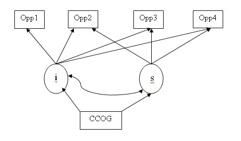
We have chosen a simple example to show how Mplus can handle growth curve modeling. Unlike most statistical software, Mplus does growth curve modeling in both long and wide format. The two approaches offer different ways of looking at the same model and offer alternative models to one another. The example here is taken from Chapter 7 of Singer and Willett’s Applied Longitudinal Data Analysis. The outcome variable is the response time on a timed cognitive task called “opposites naming”. It is measured at four time points. We will start with the long format approach. This means that each subject will have potentially four rows of observations on the dependent variable and other covariates. In other words, this is the univariate approach. This is also the standard hierarchical linear model approach.
  Data:
    File is opposites_pp.dat;
  Variable:
    Names are
       id time opp cog ccog wave;
    Missing are all (-9999) ;
    Usevariables are
       time opp ccog;
    Cluster = id;
    Within are time ;
    Between are ccog;
  Analysis: type = random twolevel;
  Model:
      %within%
      s | opp on time;
      %between%
      opp s on ccog;
      opp with s;

SUMMARY OF ANALYSIS

Number of groups                                                 1
Number of observations                                         140

Number of dependent variables                                    1
Number of independent variables                                  2
Number of continuous latent variables                            1

Observed dependent variables

  Continuous
   OPP

Observed independent variables
   TIME        CCOG

Continuous latent variables
   S

Variables with special functions

  Cluster variable      ID
  Within variables
   TIME

  Between variables
   CCOG

Estimator                                                      MLR
Information matrix                                        OBSERVED
Maximum number of iterations                                  1000
Convergence criterion                                    0.100D-05
Maximum number of EM iterations                                500
Convergence criteria for the EM algorithm
  Loglikelihood change                                   0.100D-02
  Relative loglikelihood change                          0.100D-05
  Derivative                                             0.100D-02
Minimum variance                                         0.100D-03
Maximum number of steepest descent iterations                   20
Maximum number of iterations for H1                           2000
Convergence criterion for H1                             0.100D-03
Optimization algorithm                                         EMA

Input data file(s)
  opposites_pp.dat
Input data format  FREE

SUMMARY OF DATA

     Number of clusters          35

       Size (s)    Cluster ID with Size s

          4             1      2      3      4      5      6      7      8
                        9     10     11     12     13     14     15     16
                       17     18     19     20     21     22     23     24
                       25     26     27     28     29     30     31     32
                       33     34     35

     Average cluster size   4.000

     Estimated Intraclass Correlations for the Y Variables

                Intraclass              Intraclass
     Variable  Correlation   Variable  Correlation

     OPP          0.406


THE MODEL ESTIMATION TERMINATED NORMALLY

TESTS OF MODEL FIT

Loglikelihood

          H0 Value                        -633.451
          H0 Scaling Correction Factor       0.793
            for MLR

Information Criteria

          Number of Free Parameters              8
          Akaike (AIC)                    1282.901
          Bayesian (BIC)                  1306.434
          Sample-Size Adjusted BIC        1281.123
            (n* = (n + 2) / 24)

MODEL RESULTS

                   Estimates     S.E.  Est./S.E.

Within Level

 Residual Variances
    OPP              159.727   23.491      6.800

Between Level

 S          ON
    CCOG               0.433    0.121      3.566

 OPP        ON
    CCOG              -0.114    0.416     -0.274

 OPP      WITH
    S               -165.185   67.783     -2.437

 Intercepts
    OPP              164.384    6.024     27.286
    S                 26.954    1.936     13.923

 Residual Variances
    OPP             1158.985  278.161      4.167
    S                 99.238   23.369      4.247
Example 6a. Growth curve modeling with the wide format approach
Now let’s move to growth curve modeling with a wide format approach. The data structure is now in wide format. That is each subject will only have one row of data, with four dependent variables corresponding to the four time points. In other words, this is the multivariate approach. To this end, we have to restructure the data from long to wide (in another statistical package). In order to match the results from the long format approach, we have to constrain the residual variance at each time point to be equal to each other. This also gives us a hint that the residual variances don’t have to be always equal, leading to more flexible models.
    Data:
      File is opposites_wide.dat ;
    Variable:
      Names are
         id opp1 opp2 opp3 opp4 cog ccog;
      Missing are all (-9999) ;
      usev = opp1-opp4 ccog;
    Analysis:
      Type = meanstructure;
    Model:
       i s  | opp1@0 opp2@1 opp3@2 opp4@3;
       i s on ccog;
       [i s];
       [opp1-opp4@0];   ! constraining the mean to be zero at all time points.
       opp1 - opp4 (1); ! constraining the residual variance to be equal
                        ! at all time points.
INPUT READING TERMINATED NORMALLY
SUMMARY OF ANALYSIS
Number of groups                                                 1
Number of observations                                          35
Number of dependent variables                                    4
Number of independent variables                                  1
Number of continuous latent variables                            2
Observed dependent variables
  Continuous
   OPP1        OPP2        OPP3        OPP4
Observed independent variables
   CCOG
Continuous latent variables
   I           S
Estimator                                                       ML
Information matrix                                        EXPECTED
Maximum number of iterations                                  1000
Convergence criterion                                    0.500D-04
Maximum number of steepest descent iterations                   20
Input data file(s)
  opposites_wide.dat
Input data format FREE
THE MODEL ESTIMATION TERMINATED NORMALLY
TESTS OF MODEL FIT
Chi-Square Test of Model Fit
          Value                              6.899
          Degrees of Freedom                    10
          P-Value                           0.7350
Chi-Square Test of Model Fit for the Baseline Model
          Value                            134.996
          Degrees of Freedom                    10
          P-Value                           0.0000
CFI/TLI
          CFI                                1.000
          TLI                                1.025
Loglikelihood
          H0 Value                        -770.987
          H1 Value                        -767.538
Information Criteria
          Number of Free Parameters              8
          Akaike (AIC)                    1557.975
          Bayesian (BIC)                  1570.418
          Sample-Size Adjusted BIC        1545.438
            (n* = (n + 2) / 24)
RMSEA (Root Mean Square Error Of Approximation)
          Estimate                           0.000
          90 Percent C.I.                    0.000  0.134
          Probability RMSEA <= .05           0.787
SRMR (Standardized Root Mean Square Residual)
Value 0.043
MODEL RESULTS
Estimates S.E. Est./S.E.
 I        |
    OPP1               1.000    0.000      0.000
    OPP2               1.000    0.000      0.000
    OPP3               1.000    0.000      0.000
    OPP4               1.000    0.000      0.000
 S        |
    OPP1               0.000    0.000      0.000
    OPP2               1.000    0.000      0.000
    OPP3               2.000    0.000      0.000
    OPP4               3.000    0.000      0.000
 I        ON
    CCOG              -0.114    0.489     -0.232
 S        ON
    CCOG               0.433    0.157      2.753
 S        WITH
    I               -165.303   78.279     -2.112
 Intercepts
    OPP1               0.000    0.000      0.000
    OPP2               0.000    0.000      0.000
    OPP3               0.000    0.000      0.000
    OPP4               0.000    0.000      0.000
    I                164.374    6.026     27.277
    S                 26.960    1.936     13.925
 Residual Variances
    OPP1             159.475   26.956      5.916
    OPP2             159.475   26.956      5.916
    OPP3             159.475   26.956      5.916
    OPP4             159.475   26.956      5.916
    I               1159.354  304.409      3.809
    S                 99.298   31.821      3.121
Example 6b. Growth curve modeling with the wide format approach (different parameterization)
As we have assumed in the previous models, the random intercept and the random slope are always correlated with each other. With the wide format approach, we can also model the correlation in the way of regression. This basically reparameterizes the model. But now we can describe the relationship between the intercept and the slope in terms of changes.
   Data:
      File is opposites_wide.dat ;
    Variable:
      Names are
         id opp1 opp2 opp3 opp4 cog ccog;
      Missing are all (-9999) ;
      usev = opp1-opp4 ccog;
    Analysis:
      Type = meanstructure;
    Model:
       i s  | opp1@0 opp2@1 opp3@2 opp4@3;
       i s on ccog;
       [i s];
       s on i;          ! different parameterization happens here
       [opp1-opp4@0];   ! constraining the mean to be zero at all time points.
       opp1 - opp4 (1); ! constraining the residual variance to be equal
                        ! at all time points.

TESTS OF MODEL FIT

Chi-Square Test of Model Fit

          Value                              6.899
          Degrees of Freedom                    10
          P-Value                           0.7350

Chi-Square Test of Model Fit for the Baseline Model

          Value                            134.996
          Degrees of Freedom                    10
          P-Value                           0.0000

CFI/TLI

          CFI                                1.000
          TLI                                1.025

Loglikelihood

          H0 Value                        -770.987
          H1 Value                        -767.538

Information Criteria

          Number of Free Parameters              8
          Akaike (AIC)                    1557.975
          Bayesian (BIC)                  1570.418
          Sample-Size Adjusted BIC        1545.438
            (n* = (n + 2) / 24)

RMSEA (Root Mean Square Error Of Approximation)

          Estimate                           0.000
          90 Percent C.I.                    0.000  0.134
          Probability RMSEA <= .05           0.787

SRMR (Standardized Root Mean Square Residual)

          Value                              0.043


MODEL RESULTS

                   Estimates     S.E.  Est./S.E.

 I        |
    OPP1               1.000    0.000      0.000
    OPP2               1.000    0.000      0.000
    OPP3               1.000    0.000      0.000
    OPP4               1.000    0.000      0.000

 S        |
    OPP1               0.000    0.000      0.000
    OPP2               1.000    0.000      0.000
    OPP3               2.000    0.000      0.000
    OPP4               3.000    0.000      0.000

 S        ON
    I                 -0.143    0.051     -2.773

 I        ON
    CCOG              -0.114    0.489     -0.232

 S        ON
    CCOG               0.417    0.135      3.091

 Intercepts
    OPP1               0.000    0.000      0.000
    OPP2               0.000    0.000      0.000
    OPP3               0.000    0.000      0.000
    OPP4               0.000    0.000      0.000
    I                164.374    6.026     27.277
    S                 50.398    8.613      5.852

 Residual Variances
    OPP1             159.477   26.957      5.916
    OPP2             159.477   26.957      5.916
    OPP3             159.477   26.957      5.916
    OPP4             159.477   26.957      5.916
    I               1159.380  304.416      3.809
    S                 75.726   23.268      3.255
Example 7a. Latent class analysis
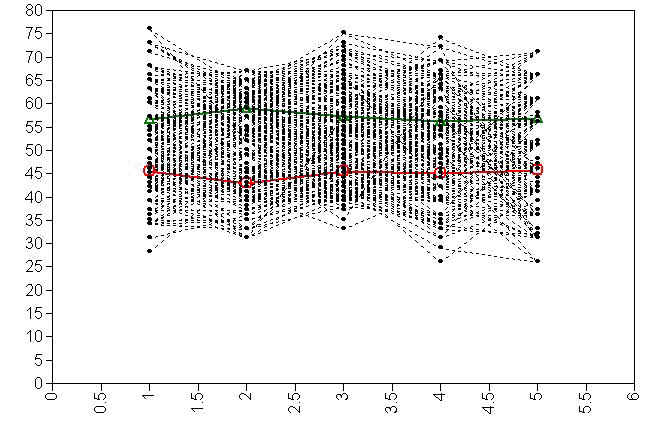
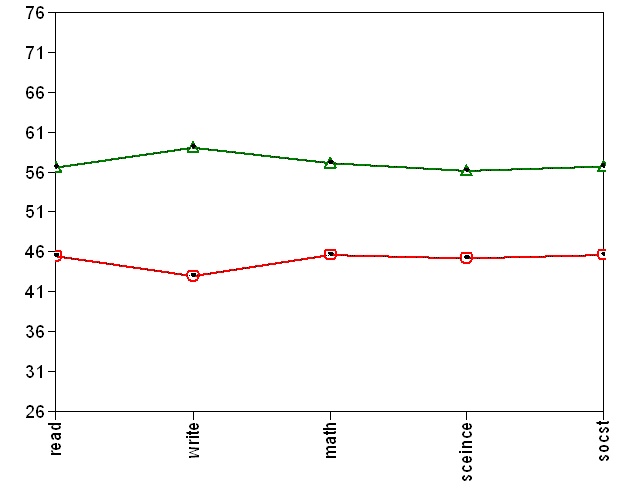
This example uses the hsb2 data set. We have test scores for the students in the sample and demographic variables as well. We want to see if we can classify students based on their test scores and how the class membership relates to other variables. This example is strictly for the purpose of illustration and therefore does not reflect any real theory or such. Notice that we have taken the default syntax to perform this analysis. We are looking for a two latent classes solution based on the scores on read, write, math, science and social studies (socst). The class membership is then regressed on the variables female and ses. Our model runs “successfully”. But Mplus gives us warning messages. It tells that the assumption that Mplus makes by default is that all the variables are uncorrelated within each latent class. Can we accept this assumption? Maybe not. But for the time being, let’s take a look at the rest of the output. We have the average scores for each of the two latent classes. We can tell that the first class has lower means on all the variables and the second one has higher means. These two classes make sense to us. Also, the class membership is highly related to ses.
  Data:
    File is hsb2.dat ;
  Variable:
    Names are
       id female race ses schtyp prog read write math science socst;
    Usevariables are
       read write math science socst female ses;
    classes = grp(2);
  Analysis:
    type=mixture;
  Model:
    %overall%
      grp#1 on female ses;

*** WARNING in Model command
  Variable is uncorrelated with all other variables within class:  READ
*** WARNING in Model command
  Variable is uncorrelated with all other variables within class:  WRITE
*** WARNING in Model command
  Variable is uncorrelated with all other variables within class:  MATH
*** WARNING in Model command
  Variable is uncorrelated with all other variables within class:  SCIENCE
*** WARNING in Model command
  Variable is uncorrelated with all other variables within class:  SOCST
*** WARNING in Model command
  All least one variable is uncorrelated with all other variables within class.
  Check that this is what is intended.
   6 WARNING(S) FOUND IN THE INPUT INSTRUCTIONS


Latent Class Analysis with Graphs

SUMMARY OF ANALYSIS

Number of groups                                                 1
Number of observations                                         200

Number of dependent variables                                    5
Number of independent variables                                  2
Number of continuous latent variables                            0
Number of categorical latent variables                           1

Observed dependent variables

  Continuous
   READ        WRITE       MATH        SCIENCE     SOCST

Observed independent variables
   FEMALE      SES

Categorical latent variables
   GRP


Estimator                                                      MLR
(output omitted...)

TESTS OF MODEL FIT

Loglikelihood

          H0 Value                       -3510.499
          H0 Scaling Correction Factor       1.126
            for MLR

Information Criteria

          Number of Free Parameters             18
          Akaike (AIC)                    7056.999
          Bayesian (BIC)                  7116.369
          Sample-Size Adjusted BIC        7059.343
            (n* = (n + 2) / 24)
          Entropy                            0.852


FINAL CLASS COUNTS AND PROPORTIONS FOR THE LATENT CLASSES
BASED ON THE ESTIMATED MODEL

    Latent
   Classes

       1         96.61160          0.48306
       2        103.38840          0.51694


FINAL CLASS COUNTS AND PROPORTIONS FOR THE LATENT CLASS PATTERNS
BASED ON ESTIMATED POSTERIOR PROBABILITIES

    Latent
   Classes

       1         96.61161          0.48306
       2        103.38839          0.51694


CLASSIFICATION OF INDIVIDUALS BASED ON THEIR MOST LIKELY LATENT CLASS MEMBERSHIP

Class Counts and Proportions

    Latent
   Classes

       1               95          0.47500
       2              105          0.52500


Average Latent Class Probabilities for Most Likely Latent Class Membership (Row)
by Latent Class (Column)

          1        2

   1   0.963    0.037
   2   0.049    0.951


MODEL RESULTS

                   Estimates     S.E.  Est./S.E.

Latent Class 1

 Means
    READ              44.645    1.107     40.336
    WRITE             45.822    1.197     38.269
    MATH              45.766    0.806     56.784
    SCIENCE           45.189    1.405     32.153
    SOCST             45.785    1.375     33.288

 Variances
    READ              50.830    5.261      9.662
    WRITE             44.222    5.109      8.656
    MATH              43.108    4.842      8.903
    SCIENCE           56.073    7.406      7.572
    SOCST             73.733    7.395      9.970

Latent Class 2

 Means
    READ              59.318    1.168     50.791
    WRITE             59.272    0.913     64.939
    MATH              59.073    1.256     47.018
    SCIENCE           58.075    0.836     69.495
    SOCST             58.591    1.041     56.288

 Variances
    READ              50.830    5.261      9.662
    WRITE             44.222    5.109      8.656
    MATH              43.108    4.842      8.903
    SCIENCE           56.073    7.406      7.572
    SOCST             73.733    7.395      9.970

Categorical Latent Variables

 GRP#1      ON
    FEMALE            -0.173    0.344     -0.502
    SES               -0.779    0.222     -3.506

 Intercepts
    GRP#1              1.622    0.556      2.917


LOGISTIC REGRESSION ODDS RATIO RESULTS

Categorical Latent Variables

 GRP#1    ON
    FEMALE             0.841
    SES                0.459


ALTERNATIVE PARAMETERIZATIONS FOR THE CATEGORICAL LATENT VARIABLE REGRESSION

Parameterization using Reference Class 1

 GRP#2    ON
    FEMALE             0.173    0.344      0.502
    SES                0.779    0.222      3.506

 Intercepts
    GRP#2             -1.622    0.556     -2.917
Example 7b. Latent class analysis with graphics
Now, let’s take up the issue of the correlation of variables within latent classes. We will also request some plots. Should we allow all the test scores to be correlated with each other? Maybe not. In this example, we allow reading scores to be correlated with all the other test scores, writing scores to be correlated with social studies scores, and math scores to be correlated with the science scores. We can take a look at the difference in AIC values and conclude that this is a better fitting model than the previous one.
    Data:
      File is hsb2.dat ;
    Variable:
      Names are
         id female race ses schtyp prog read write math science socst;
      Usevariables are
         read write math science socst female ses;
      classes = grp(2);
    Analysis:
      type=mixture;
    Model:
      %overall%
        read with write;
        read with math;
        read with science;
        read with socst;

        write with socst;

        math with science;

        grp#1 on female ses;
    Plot:
       type is plot3;
       series is read (1) write (2) math (3) science (4) socst (5);

(output omitted...)

TESTS OF MODEL FIT

Loglikelihood

          H0 Value                       -3455.156
          H0 Scaling Correction Factor       1.068
            for MLR

Information Criteria

          Number of Free Parameters             24
          Akaike (AIC)                    6958.313
          Bayesian (BIC)                  7037.472
          Sample-Size Adjusted BIC        6961.438
            (n* = (n + 2) / 24)
          Entropy                            0.838

FINAL CLASS COUNTS AND PROPORTIONS FOR THE LATENT CLASSES
BASED ON THE ESTIMATED MODEL

    Latent
   Classes

       1         77.82126          0.38911
       2        122.17874          0.61089


FINAL CLASS COUNTS AND PROPORTIONS FOR THE LATENT CLASS PATTERNS
BASED ON ESTIMATED POSTERIOR PROBABILITIES

    Latent
   Classes

       1         77.82125          0.38911
       2        122.17875          0.61089


CLASSIFICATION OF INDIVIDUALS BASED ON THEIR MOST LIKELY LATENT CLASS MEMBERSHIP

Class Counts and Proportions

    Latent
   Classes

       1               76          0.38000
       2              124          0.62000


Average Latent Class Probabilities for Most Likely Latent Class Membership (Row)
by Latent Class (Column)

          1        2

   1   0.956    0.044
   2   0.042    0.958


MODEL RESULTS

                   Estimates     S.E.  Est./S.E.

Latent Class 1

 READ     WITH
    WRITE              9.024    3.276      2.755
    MATH              24.570    5.285      4.649
    SCIENCE           27.390    5.820      4.706
    SOCST             25.783    5.457      4.724

 WRITE    WITH
    SOCST             18.927    3.559      5.319

 MATH     WITH
    SCIENCE           27.609    6.718      4.109

 Means
    READ              45.417    0.942     48.209
    WRITE             42.995    1.347     31.917
    MATH              45.527    0.722     63.091
    SCIENCE           45.100    1.172     38.487
    SOCST             45.613    1.261     36.185

 Variances
    READ              66.360    5.860     11.324
    WRITE             28.467    4.359      6.530
    MATH              55.061    6.780      8.121
    SCIENCE           68.513    9.495      7.216
    SOCST             85.301    8.522     10.010

Latent Class 2

 READ     WITH
    WRITE              9.024    3.276      2.755
    MATH              24.570    5.285      4.649
    SCIENCE           27.390    5.820      4.706
    SOCST             25.783    5.457      4.724

 WRITE    WITH
    SOCST             18.927    3.559      5.319

 MATH     WITH
    SCIENCE           27.609    6.718      4.109

 Means
    READ              56.570    1.153     49.054
    WRITE             59.005    0.580    101.768
    MATH              57.179    1.072     53.347
    SCIENCE           56.150    1.018     55.171
    SOCST             56.731    1.024     55.428

 Variances
    READ              66.360    5.860     11.324
    WRITE             28.467    4.359      6.530
    MATH              55.061    6.780      8.121
    SCIENCE           68.513    9.495      7.216
    SOCST             85.301    8.522     10.010

Categorical Latent Variables

 GRP#1      ON
    FEMALE            -1.166    0.419     -2.780
    SES               -1.069    0.278     -3.842

 Intercepts
    GRP#1              2.297    0.665      3.456


LOGISTIC REGRESSION ODDS RATIO RESULTS

Categorical Latent Variables

 GRP#1    ON
    FEMALE             0.312
    SES                0.343


ALTERNATIVE PARAMETERIZATIONS FOR THE CATEGORICAL LATENT VARIABLE REGRESSION

Parameterization using Reference Class 1

 GRP#2    ON
    FEMALE             1.166    0.419      2.780
    SES                1.069    0.278      3.842

 Intercepts
    GRP#2             -2.297    0.665     -3.456