Mplus version 5.2 was used for these examples.
1.0 Descriptive statistics in Mplus
To indicate to Mplus that you want basic descriptive statistics (means, variances, covariances and correlations), you need to enter Type = basic; in the analysis command block. If you would like to be able to view histograms or scatterplots of some of your variables, you can add a plot command block. These types of univariate and bivariate graphs are plot1 types of graphs.
The data set is https://stats.idre.ucla.edu/wp-content/uploads/2016/02/hsb-1.dat .
Title:
  Entering data example free format using https://stats.idre.ucla.edu/wp-content/uploads/2016/02/hsb-1.dat
Data:
  File is "D:/https://stats.idre.ucla.edu/wp-content/uploads/2016/02/hsb-1.dat";
Variable:
  Names are
    id female race ses schtyp prog read write math science socst;
  Usevariables are
    id female race ses schtyp prog read write math science socst;
Analysis:
  Type = basic;
Plot:
  Type is plot1;
Here is the output that Mplus generates.
SUMMARY OF ANALYSIS

Number of groups                                                 1
Number of observations                                         200

Number of dependent variables                                   11
Number of independent variables                                  0
Number of continuous latent variables                            0

Observed dependent variables

  Continuous
   READ        WRITE       MATH        ID          FEMALE      RACE
   SES         SCHTYP      PROG        SCIENCE     SOCST


Estimator                                                       ML
Information matrix                                        OBSERVED
Maximum number of iterations                                  1000
Convergence criterion                                    0.500D-04
Maximum number of steepest descent iterations                   20

Input data file(s)
  D:/https://stats.idre.ucla.edu/wp-content/uploads/2016/02/hsb-1.dat

Input data format  FREE

RESULTS FOR BASIC ANALYSIS


     SAMPLE STATISTICS


           Means
              READ          WRITE         MATH          ID            FEMALE
              ________      ________      ________      ________      ________
      1        52.230        52.775        52.645       100.500         0.545


           Means
              RACE          SES           SCHTYP        PROG          SCIENCE
              ________      ________      ________      ________      ________
      1         3.430         2.055         1.160         2.025        51.850


           Means
              SOCST
              ________
      1        52.405


           Covariances
              READ          WRITE         MATH          ID            FEMALE
              ________      ________      ________      ________      ________
 READ         105.123
 WRITE         57.997        89.844
 MATH          63.615        54.829        87.768
 ID            88.196       102.420       118.877      3350.000
 FEMALE        -0.272         1.214        -0.137        -2.520         0.249
 RACE           2.594         2.168         1.973        45.050         0.001
 SES            2.178         1.424         1.849         8.842        -0.045
 SCHTYP         0.325         0.443         0.338        10.261         0.003
 PROG          -0.956        -1.185        -0.971        -2.319         0.001
 SCIENCE       63.969        53.534        58.504       184.181        -0.631
 SOCST         68.409        61.544        54.763       113.902         0.281


           Covariances
              RACE          SES           SCHTYP        PROG          SCIENCE
              ________      ________      ________      ________      ________
 RACE           1.081
 SES            0.147         0.525
 SCHTYP         0.041         0.036         0.135
 PROG          -0.036         0.009        -0.024         0.477
 SCIENCE        3.296         2.028         0.235        -1.298        98.028
 SOCST          2.121         2.581         0.382        -1.447        49.438


           Covariances
              SOCST
              ________
 SOCST        115.257


           Correlations
              READ          WRITE         MATH          ID            FEMALE
              ________      ________      ________      ________      ________
 READ           1.000
 WRITE          0.597         1.000
 MATH           0.662         0.617         1.000
 ID             0.149         0.187         0.219         1.000
 FEMALE        -0.053         0.256        -0.029        -0.087         1.000
 RACE           0.243         0.220         0.203         0.749         0.001
 SES            0.293         0.207         0.272         0.211        -0.125
 SCHTYP         0.086         0.127         0.098         0.482         0.015
 PROG          -0.135        -0.181        -0.150        -0.058         0.004
 SCIENCE        0.630         0.570         0.631         0.321        -0.128
 SOCST          0.621         0.605         0.544         0.183         0.052


           Correlations
              RACE          SES           SCHTYP        PROG          SCIENCE
              ________      ________      ________      ________      ________
 RACE           1.000
 SES            0.195         1.000
 SCHTYP         0.108         0.137         1.000
 PROG          -0.050         0.017        -0.095         1.000
 SCIENCE        0.320         0.283         0.065        -0.190         1.000
 SOCST          0.190         0.332         0.097        -0.195         0.465


           Correlations
              SOCST
              ________
 SOCST          1.000


PLOT INFORMATION

The following plots are available:

  Histograms (sample values)
  Scatterplots (sample values)

     Beginning Time:  11:35:42
        Ending Time:  11:35:43
       Elapsed Time:  00:00:01
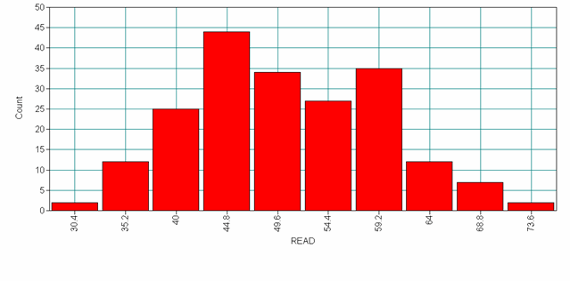
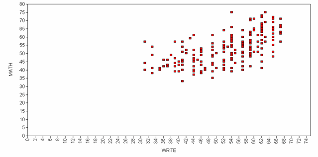
You can compare these summary statistics to those found in another software package or by hand to ensure that you have read the data into Mplus correctly. To view plots, you can select Graph, View graphs or press Alt-V to open the dialog box below.
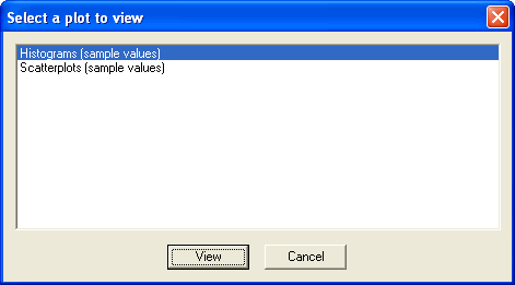
From here, you can select Histograms and choose read from the drop down menu to get the plot below.
Alternatively, you can select Scatterplots and choose to look at math and write.
2.0 Descriptive statistics with missing data without listwise deletion
Next, we will look at a dataset with missing data. This time we will not include the id variable in the analyses. We will use the hsbmis.dat datafile and hsbmis.inp command file created by Stata in the previous section to demonstrate the descriptive statistics.
Data:
  File is "D:hsbmis.dat" ;
Variable:
  Names are
     id female race ses schtyp prog read write math science socst;
  Missing are all (-9999) ;
  Usevariables are
     female race ses schtyp prog read write math science socst;
  Analysis:
    type = basic missing ; ! note we added missing
Here is the output generated by Mplus.
SUMMARY OF ANALYSIS

Number of groups                                                 1
Number of observations                                         200

Number of dependent variables                                   11
Number of independent variables                                  0
Number of continuous latent variables                            0

Observed dependent variables

  Continuous
   ID          FEMALE      RACE        SES         SCHTYP      PROG
   READ        WRITE       MATH        SCIENCE     SOCST


Estimator                                                       ML
Information matrix                                        OBSERVED
Maximum number of iterations                                  1000
Convergence criterion                                    0.500D-04
Maximum number of steepest descent iterations                   20
Maximum number of iterations for H1                           2000
Convergence criterion for H1                             0.100D-03

Input data file(s)
  D:hsbmis.dat

Input data format  FREE


SUMMARY OF DATA

     Number of missing data patterns             7


SUMMARY OF MISSING DATA PATTERNS


     MISSING DATA PATTERNS (x = not missing)

           1  2  3  4  5  6  7
 ID        x  x  x  x  x  x  x
 FEMALE    x  x  x  x  x  x
 RACE      x  x  x  x  x  x  x
 SES       x  x  x  x  x  x  x
 SCHTYP    x  x  x  x  x  x  x
 PROG      x  x  x  x  x  x  x
 READ      x  x  x  x  x     x
 WRITE     x  x  x  x     x  x
 MATH      x  x  x     x  x  x
 SCIENCE   x  x     x  x  x  x
 SOCST     x     x  x  x  x  x


     MISSING DATA PATTERN FREQUENCIES

    Pattern   Frequency     Pattern   Frequency     Pattern   Frequency
          1         138           4          12           7           6
          2           5           5          14
          3          14           6          11


COVARIANCE COVERAGE OF DATA

Minimum covariance coverage value   0.100


     PROPORTION OF DATA PRESENT


           Covariance Coverage
              ID            FEMALE        RACE          SES           SCHTYP
              ________      ________      ________      ________      ________
 ID             1.000
 FEMALE         0.970         0.970
 RACE           1.000         0.970         1.000
 SES            1.000         0.970         1.000         1.000
 SCHTYP         1.000         0.970         1.000         1.000         1.000
 PROG           1.000         0.970         1.000         1.000         1.000
 READ           0.945         0.915         0.945         0.945         0.945
 WRITE          0.930         0.900         0.930         0.930         0.930
 MATH           0.940         0.910         0.940         0.940         0.940
 SCIENCE        0.930         0.900         0.930         0.930         0.930
 SOCST          0.975         0.945         0.975         0.975         0.975


           Covariance Coverage
              PROG          READ          WRITE         MATH          SCIENCE
              ________      ________      ________      ________      ________
 PROG           1.000
 READ           0.945         0.945
 WRITE          0.930         0.875         0.930
 MATH           0.940         0.885         0.870         0.940
 SCIENCE        0.930         0.875         0.860         0.870         0.930
 SOCST          0.975         0.920         0.905         0.915         0.905


           Covariance Coverage
              SOCST
              ________
 SOCST          0.975


RESULTS FOR BASIC ANALYSIS


     ESTIMATED SAMPLE STATISTICS


           Means
              ID            FEMALE        RACE          SES           SCHTYP
              ________      ________      ________      ________      ________
      1       100.500         0.546         3.430         2.055         1.160


           Means
              PROG          READ          WRITE         MATH          SCIENCE
              ________      ________      ________      ________      ________
      1         2.025        52.361        52.560        52.796        51.839


           Means
              SOCST
              ________
      1        52.353


           Covariances
              ID            FEMALE        RACE          SES           SCHTYP
              ________      ________      ________      ________      ________
 ID          3333.250
 FEMALE        -1.848         0.247
 RACE          44.825         0.015         1.075
 SES            8.797        -0.041         0.146         0.522
 SCHTYP        10.210         0.002         0.041         0.036         0.134
 PROG          -2.308         0.008        -0.036         0.009        -0.024
 READ          87.947        -0.281         2.622         2.285         0.350
 WRITE        100.623         1.199         2.052         1.386         0.475
 MATH         120.213        -0.249         2.086         1.680         0.240
 SCIENCE      168.152        -0.602         3.084         1.861         0.290
 SOCST        113.330         0.252         2.035         2.546         0.388


           Covariances
              PROG          READ          WRITE         MATH          SCIENCE
              ________      ________      ________      ________      ________
 PROG           0.474
 READ          -0.964       104.529
 WRITE         -1.197        56.743        88.262
 MATH          -1.117        61.541        53.418        84.921
 SCIENCE       -1.456        63.739        54.726        58.634        94.130
 SOCST         -1.432        67.903        60.147        50.856        50.528


           Covariances
              SOCST
              ________
 SOCST        115.411


           Correlations
              ID            FEMALE        RACE          SES           SCHTYP
              ________      ________      ________      ________      ________
 ID             1.000
 FEMALE        -0.064         1.000
 RACE           0.749         0.029         1.000
 SES            0.211        -0.114         0.195         1.000
 SCHTYP         0.482         0.013         0.108         0.137         1.000
 PROG          -0.058         0.023        -0.050         0.017        -0.095
 READ           0.149        -0.055         0.247         0.309         0.093
 WRITE          0.186         0.256         0.211         0.204         0.138
 MATH           0.226        -0.054         0.218         0.252         0.071
 SCIENCE        0.300        -0.125         0.307         0.265         0.082
 SOCST          0.183         0.047         0.183         0.328         0.099


           Correlations
              PROG          READ          WRITE         MATH          SCIENCE
              ________      ________      ________      ________      ________
 PROG           1.000
 READ          -0.137         1.000
 WRITE         -0.185         0.591         1.000
 MATH          -0.176         0.653         0.617         1.000
 SCIENCE       -0.218         0.643         0.600         0.656         1.000
 SOCST         -0.194         0.618         0.596         0.514         0.485


           Correlations
              SOCST
              ________
 SOCST          1.000


     MAXIMUM LOG-LIKELIHOOD VALUE FOR THE UNRESTRICTED (H1) MODEL IS   -5102.296


     Beginning Time:  11:56:08
        Ending Time:  11:56:08
       Elapsed Time:  00:00:00
Because we indicated that our data included missing values, our basic output included “SUMMARY OF MISSING DATA PATTERNS” in which we can see which combinations of variables are missing for how many observations in our data. From this section of output, we can see that we have 138 complete observations and no more than one missing variable in any of our other observations.
2.1 Descriptive statistics with missing data with listwise deletion
You might also notice that the descriptive statistics from Mplus do not match with the output from a standard statistics software package, such as SPSS, Stata or SAS, when missing data are present. This is because that by default Mplus uses the maximum likelihood estimation, and it uses all the available values instead of doing the listwise deletion, which is the default behavior in SPSS, Stata or SAS. For the purpose of checking data, you can request that Mplus does listwise deletion as well. Here is the syntax.
Data:
  File is "D:hsbmis.dat" ;
  listwise = on;
Variable:
  Names are
     id female race ses schtyp prog read write math science socst;
  Missing are all (-9999) ;
  Usevariables are
     female race ses schtyp prog read write math science socst;
  Analysis:
    type = basic ;