
Purpose: The following page will explain how to perform a latent class analysis in Mplus, one with categorical variables and the other with a mix of categorical and continuous variables. A mixture model with categorical variables is called latent class analysis, whereas a mixture model with only continuous variables is called a latent profile analysis (Oberski, 2016).
Note: Mplus version 8 was used for these examples. Download all the files for this portion of this seminar.
1.0 Basic latent class analysis model
Latent class analysis is used to classify individuals into homogeneous subgroups. Individual differences in observed item response patterns are explained by differences in latent class membership (Geiser, 2013). For the case with only dichotomous variables \(X=\{0,1\}\), the latent class analysis (LCA) model for a single item can be written as:
$$
P(X_{vi} =1) = \sum_{g=1}^{G} \pi_{g} \pi_{ig}
$$
where \(P(X_{vi}=1)\) denotes the unconditional probability that a randomly selected individual \(v\) obtained a score of \(X=1\) on item \(i\), \((i=1,\cdots,I)\) and the parameter
$$
\pi_{ig} = P(X_{vi} = 1 | G = g)
$$
is the conditional solution probability. Since the sum of the two conditional probabilities equals one,
$$
P(X_{vi} = 0 | G = g) = 1-\pi_{ig}.
$$
The class size parameter \(\pi_g\) indicates the unconditional probability of belonging to latent class \(g\), \((g = 1, \cdots, G)\), and the sum of all class-size parameters is 1, i.e.,
$$
\sum_{g=1}^{G} \pi_{g} = 1.
$$
We will illustrate a simple latent class analysis (LCA) using the mplus73recode.dat dataset and see if we can identify two classes based on four binary variables. For example, the variable u1 indicates whether the student was in honors math in seventh grade (1=yes; 0=no); the variable u2 indicates whether the student was in honors math in eighth grade; rc3 indicates whether the student was in honors math in ninth grade; and rc4 indicates whether the student was in honors math in tenth grade. We specify that two latent classes should be extracted, and we expect that these classes will differentiate students who have a particularly high aptitude in math from those who do not.
In the syntax below, the title statement is used to remind us what analysis we are running. The data statement tells Mplus where the text data file is located. The variables statement tells Mplus the names of the variables in the text file (these names are not listed at the top of the text file); the usevariables statement tells Mplus which variables we will be using in this analysis; the classes statement indicates the number of classes we wish to extract; and the categorical statement tells Mplus which variables are categorical.
By specifying mixture on the analysis statement, we tell Mplus that our data are a mixture of two subpopulations. We use the savedata
statement save to class membership information to a text file called lca73classes.txt. We will save the class probabilities (cprob) in this file, and the file will be a free format text file. We can open this file in another program and look at the class membership probabilities and class assignment. The plot statement requests that we would like get all possible plots (type 3), graphs where the values are connected by a line. The (*) at the end of the series statement requests integer values starting with 0 and increasing by 1.
title:  This is an example of LCA with binary latent class indicators

data:
    file is mplus73recode.dat;

variable:
    names are u1-u4 rc3 rc4 x1-x10;
    usevariables = u1 u2 rc3 rc4;
    classes = c (2);
    categorical = u1 u2 rc3 rc4;

analysis:
    type=mixture;

savedata:
    file is lca73classes.txt ;
    save is cprob;
    format is free;

plot:
    type is plot3;
    series is u1 u2 rc3 rc4(*);
Below is the resulting output.
SUMMARY OF ANALYSIS

Number of groups                                                 1
Number of observations                                         500

Number of dependent variables                                    4
Number of independent variables                                  0
Number of continuous latent variables                            0
Number of categorical latent variables                           1

Observed dependent variables

  Binary and ordered categorical (ordinal)
   U1          U2          RC3         RC4

Categorical latent variables
   C


Estimator                                                      MLR
Information matrix                                        OBSERVED
Optimization Specifications for the Quasi-Newton Algorithm for
Continuous Outcomes
  Maximum number of iterations                                 100
  Convergence criterion                                  0.100D-05
Optimization Specifications for the EM Algorithm
  Maximum number of iterations                                 500
  Convergence criteria
    Loglikelihood change                                 0.100D-06
    Relative loglikelihood change                        0.100D-06
    Derivative                                           0.100D-05
Optimization Specifications for the M step of the EM Algorithm for
Categorical Latent variables
  Number of M step iterations                                    1
  M step convergence criterion                           0.100D-05
  Basis for M step termination                           ITERATION
Optimization Specifications for the M step of the EM Algorithm for
Censored, Binary or Ordered Categorical (Ordinal), Unordered
Categorical (Nominal) and Count Outcomes
  Number of M step iterations                                    1
  M step convergence criterion                           0.100D-05
  Basis for M step termination                           ITERATION
  Maximum value for logit thresholds                            15
  Minimum value for logit thresholds                           -15
  Minimum expected cell size for chi-square              0.100D-01
Optimization algorithm                                         EMA
Random Starts Specifications
  Number of initial stage random starts                         10
  Number of final stage optimizations                            2
  Number of initial stage iterations                            10
  Initial stage convergence criterion                    0.100D+01
  Random starts scale                                    0.500D+01
  Random seed for generating random starts                       0
Link                                                         LOGIT

Input data file(s)
  d:datamplus73recode.dat
Input data format  FREE


SUMMARY OF CATEGORICAL DATA PROPORTIONS

    U1
      Category 1    0.678
      Category 2    0.322
    U2
      Category 1    0.686
      Category 2    0.314
    RC3
      Category 1    0.678
      Category 2    0.322
    RC4
      Category 1    0.666
      Category 2    0.334


RANDOM STARTS RESULTS RANKED FROM THE BEST TO THE WORST LOGLIKELIHOOD VALUES

Final stage loglikelihood values at local maxima, seeds, and initial stage start numbers:

            -965.244  253358           2
            -965.244  285380           1

THE MODEL ESTIMATION TERMINATED NORMALLY

TESTS OF MODEL FIT

Loglikelihood

          H0 Value                        -965.244
          H0 Scaling Correction Factor       1.013
            for MLR

Information Criteria

          Number of Free Parameters              9
          Akaike (AIC)                    1948.488
          Bayesian (BIC)                  1986.420
          Sample-Size Adjusted BIC        1957.853
            (n* = (n + 2) / 24)

Chi-Square Test of Model Fit for the Binary and Ordered Categorical
(Ordinal) Outcomes

          Pearson Chi-Square

          Value                              6.287
          Degrees of Freedom                     6
          P-Value                           0.3918

          Likelihood Ratio Chi-Square

          Value                              5.605
          Degrees of Freedom                     6
          P-Value                           0.4688

FINAL CLASS COUNTS AND PROPORTIONS FOR THE LATENT CLASSES
BASED ON THE ESTIMATED MODEL

    Latent
   Classes

       1        136.38034          0.27276
       2        363.61966          0.72724

FINAL CLASS COUNTS AND PROPORTIONS FOR THE LATENT CLASS PATTERNS
BASED ON ESTIMATED POSTERIOR PROBABILITIES

    Latent
   Classes

       1        136.38059          0.27276
       2        363.61941          0.72724


CLASSIFICATION QUALITY

     Entropy                         0.904

CLASSIFICATION OF INDIVIDUALS BASED ON THEIR MOST LIKELY LATENT CLASS MEMBERSHIP

Class Counts and Proportions

    Latent
   Classes

       1              127          0.25400
       2              373          0.74600

Average Latent Class Probabilities for Most Likely Latent Class Membership (Row)
by Latent Class (Column)

           1        2

    1   0.986    0.014
    2   0.030    0.970

MODEL RESULTS

                                                    Two-Tailed
                    Estimate       S.E.  Est./S.E.    P-Value

Latent Class 1

 Thresholds
    U1$1              -2.063      0.373     -5.536      0.000
    U2$1              -1.724      0.300     -5.755      0.000
    RC3$1             -2.331      0.390     -5.985      0.000
    RC4$1             -2.078      0.320     -6.490      0.000

Latent Class 2

 Thresholds
    U1$1               2.091      0.182     11.502      0.000
    U2$1               2.056      0.180     11.401      0.000
    RC3$1              2.187      0.203     10.760      0.000
    RC4$1              1.937      0.183     10.613      0.000

Categorical Latent Variables

 Means
    C#1               -0.981      0.116     -8.468      0.000


RESULTS IN PROBABILITY SCALE

Latent Class 1

 U1
    Category 1         0.113      0.037      3.024      0.002
    Category 2         0.887      0.037     23.800      0.000
 U2
    Category 1         0.151      0.038      3.934      0.000
    Category 2         0.849      0.038     22.056      0.000
 RC3
    Category 1         0.089      0.031      2.817      0.005
    Category 2         0.911      0.031     28.987      0.000
 RC4
    Category 1         0.111      0.032      3.514      0.000
    Category 2         0.889      0.032     28.072      0.000

Latent Class 2

 U1
    Category 1         0.890      0.018     50.016      0.000
    Category 2         0.110      0.018      6.181      0.000
 U2
    Category 1         0.887      0.018     48.873      0.000
    Category 2         0.113      0.018      6.256      0.000
 RC3
    Category 1         0.899      0.018     48.748      0.000
    Category 2         0.101      0.018      5.472      0.000
 RC4
    Category 1         0.874      0.020     43.498      0.000
    Category 2         0.126      0.020      6.267      0.000

LATENT CLASS ODDS RATIO RESULTS

Latent Class 1 Compared to Latent Class 2

 U1
    Category > 1      63.673     25.877      2.461      0.014
 U2
    Category > 1      43.796     14.941      2.931      0.003
 RC3
    Category > 1      91.672     38.990      2.351      0.019
 RC4
    Category > 1      55.439     20.032      2.768      0.006

QUALITY OF NUMERICAL RESULTS

     Condition Number for the Information Matrix              0.600E-01
       (ratio of smallest to largest eigenvalue)

PLOT INFORMATION

The following plots are available:

  Histograms (sample values)
  Scatterplots (sample values)
  Sample proportions
  Estimated probabilities

SAVEDATA INFORMATION

  Order of variables

    U1
    U2
    RC3
    RC4
    CPROB1
    CPROB2
    C

  Save file
    lca73classes.txt

  Save file format           Free

  Save file record length    5000
To view the graphs, click on Graph and then View Graphs. From the list,
we selected Estimated Probabilities.
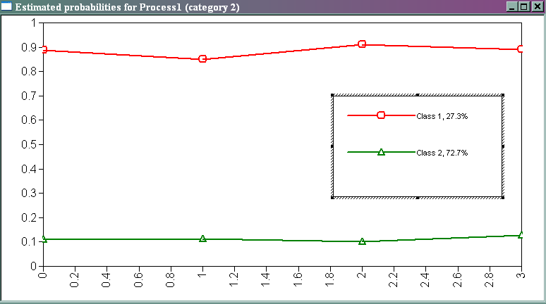
The graph above corresponds to the table in the output entitled “Results in Probability Scale”. As you can see in the title bar of the graph, the plotted points are for category 2. The y-axis is the probability, and the x-axis gives the four binary predictor variables. The variable u1
is called 0, the variable u2 is called 1, the variable rc3 is called 2, and the variable rc4 is called 3. The labeling of the x-axis starts at 0 and increases in increments of 1 because of the way we specified the series statement. We used simple syntax that did not yield a simple labeling of the x-axis.
We can see from the legend in the middle of the graph that 27.3% of this sample of students is in latent class 1, while 72.7% of the sample of students is in latent class 2. This information can be found in the table in the output entitled “Final Class Counts and Proportions for the latent Classes Based on the Estimated Model”.
The red line indicates latent class 1, which we believe is the class containing the gifted math students. Students in latent class 1 have a
probability of 0.887 of having a value of 1 on the variable u1 (being in honors math in seventh grade). The green line indicates latent class 2, which we believe is the class containing the regular math students. The probability that a student in latent class 2 has value of 1 on the variable u1 is .110. The probability that a student in latent class 1 has a value of 1 on the variable u2 (being in honors math in the eighth grade) is 0.849, while the probability that a student in latent class 2 has a value of 1 on the variable u2 is only 0.113. As you can see from the graph, the students in latent class 1 have a high probability of having a value on all of the binary variables. Remember that a value of 1 on these variables indicates that the student was in honors math in that grade.
If we look at the the first few cases in the outputted file that we requested, we can see that the output and graph correspond to this file.
The outputted text file does not contain variable names, but you can find this information in the output in the table entitled “Savedata Information” (towards the end of the output). This tells us that the first four variables are the observed binary variables from our mplus73recode data file, the next variable is class probability 1, then class probability 2, and the last variable (called c), is the assigned class membership. The first two students have very high probabilities for class 1 and low probabilities for class 2, and they are assigned to class 1. The last two students whose data are listed below were in no honors math classes; they have 0 probability of being in class 1, a 1.0 probability of being in class 2, and they are in class 2.
     1.000      1.000      1.000      0.000      0.963      0.037      1.000
     1.000      0.000      1.000      1.000      0.971      0.029      1.000
     0.000      0.000      0.000      0.000      0.000      1.000      2.000
     1.000      1.000      1.000      1.000      0.999      0.001      1.000
     1.000      1.000      1.000      1.000      0.999      0.001      1.000
     0.000      1.000      0.000      0.000      0.004      0.996      2.000
     1.000      1.000      1.000      1.000      0.999      0.001      1.000
     0.000      0.000      0.000      0.000      0.000      1.000      2.000
     0.000      0.000      0.000      1.000      0.006      0.994      2.000
     0.000      0.000      0.000      0.000      0.000      1.000      2.000
     0.000      0.000      0.000      1.000      0.006      0.994      2.000
     0.000      0.000      0.000      0.000      0.000      1.000      2.000
     0.000      0.000      0.000      0.000      0.000      1.000      2.000
     1.000      1.000      1.000      1.000      0.999      0.001      1.000
     0.000      0.000      0.000      0.000      0.000      1.000      2.000
     0.000      0.000      0.000      0.000      0.000      1.000      2.000
2.0 Using both categorical and continuous predictor variables
When modeling latent variables, you can use any combination of categorical and continuous variables. In this example, we will use both categorical and continuous variables.
title:  Both categorical and continuous variables

data:
     file is mplus73recode.dat;

variable:
    names are u1-u4 rc3 rc4 x1-x10;
    usevar are u1 u2 rc3 rc4 x1 - x5;
    categorical are u1 u2 rc3 rc4;
    classes = grp (2);

analysis:
    type = mixture;
plot:
    type is plot3;
    series is  x1-x3(*);
As you can see, the syntax is very similar to the previous example. We have five continuous variables listed on the usevariables statement (which was shorted to usevar). The name of the classes was changed to grp (you can name it anything that you want), and we again asked for plots. Please note that when you request plots, you can specify plots for either categorical or continuous variable, but not for both. Also, the types of plots available depend on the model specified. If you specify the model such that the latent classes are determined by one set of predictors and the class membership is determined by a different set of predictors, then you can get a larger variety of graphs.
Below is the abbreviated output.
*** WARNING in MODEL command
  All variables are uncorrelated with all other variables within class.
  Check that this is what is intended.
   1 WARNING(S) FOUND IN THE INPUT INSTRUCTIONS

Both categorical and continuous variables

SUMMARY OF ANALYSIS

Number of groups                                                 1
Number of observations                                         500

Number of dependent variables                                    9
Number of independent variables                                  0
Number of continuous latent variables                            0
Number of categorical latent variables                           1

Observed dependent variables

  Continuous
   X1          X2          X3          X4          X5

  Binary and ordered categorical (ordinal)
   U1          U2          RC3         RC4

Categorical latent variables
   GRP

THE MODEL ESTIMATION TERMINATED NORMALLY

TESTS OF MODEL FIT

Loglikelihood

          H0 Value                       -4567.250
          H0 Scaling Correction Factor       0.987
            for MLR

Information Criteria

          Number of Free Parameters             24
          Akaike (AIC)                    9182.500
          Bayesian (BIC)                  9283.651
          Sample-Size Adjusted BIC        9207.474
            (n* = (n + 2) / 24)

Chi-Square Test of Model Fit for the Binary and Ordered Categorical
(Ordinal) Outcomes

          Pearson Chi-Square

          Value                              7.629
          Degrees of Freedom                     6
          P-Value                           0.2665

          Likelihood Ratio Chi-Square

          Value                              6.974
          Degrees of Freedom                     6
          P-Value                           0.3233

FINAL CLASS COUNTS AND PROPORTIONS FOR THE LATENT CLASSES
BASED ON THE ESTIMATED MODEL

    Latent
   Classes

       1        367.57723          0.73515
       2        132.42277          0.26485

FINAL CLASS COUNTS AND PROPORTIONS FOR THE LATENT CLASS PATTERNS
BASED ON ESTIMATED POSTERIOR PROBABILITIES

    Latent
   Classes

       1        367.57724          0.73515
       2        132.42276          0.26485


CLASSIFICATION QUALITY

     Entropy                         0.998

CLASSIFICATION OF INDIVIDUALS BASED ON THEIR MOST LIKELY LATENT CLASS MEMBERSHIP

Class Counts and Proportions

    Latent
   Classes

       1              368          0.73600
       2              132          0.26400


Average Latent Class Probabilities for Most Likely Latent Class Membership (Row)
by Latent Class (Column)

           1        2

    1   0.999    0.001
    2   0.000    1.000

MODEL RESULTS

                                                    Two-Tailed
                    Estimate       S.E.  Est./S.E.    P-Value

Latent Class 1

 Means
    X1                -2.058      0.055    -37.120      0.000
    X2                -2.061      0.051    -40.653      0.000
    X3                -0.987      0.055    -18.069      0.000
    X4                -0.990      0.052    -19.020      0.000
    X5                -0.040      0.053     -0.759      0.448

 Thresholds
    U1$1               2.021      0.162     12.454      0.000
    U2$1               2.075      0.166     12.521      0.000
    RC3$1              2.075      0.166     12.526      0.000
    RC4$1              1.930      0.157     12.279      0.000

 Variances
    X1                 1.116      0.073     15.348      0.000
    X2                 0.956      0.058     16.600      0.000
    X3                 1.031      0.059     17.382      0.000
    X4                 0.946      0.060     15.722      0.000
    X5                 1.064      0.067     15.762      0.000

Latent Class 2

 Means
    X1                 1.988      0.091     21.874      0.000
    X2                 1.971      0.087     22.659      0.000
    X3                 0.987      0.081     12.249      0.000
    X4                 0.829      0.080     10.424      0.000
    X5                 0.097      0.095      1.022      0.307

 Thresholds
    U1$1              -2.102      0.283     -7.440      0.000
    U2$1              -1.955      0.266     -7.353      0.000
    RC3$1             -2.268      0.302     -7.516      0.000
    RC4$1             -2.306      0.303     -7.617      0.000

 Variances
    X1                 1.116      0.073     15.348      0.000
    X2                 0.956      0.058     16.600      0.000
    X3                 1.031      0.059     17.382      0.000
    X4                 0.946      0.060     15.722      0.000
    X5                 1.064      0.067     15.762      0.000

Categorical Latent Variables

 Means
    GRP#1              1.021      0.102     10.056      0.000

RESULTS IN PROBABILITY SCALE

Latent Class 1

 U1
    Category 1         0.883      0.017     52.667      0.000
    Category 2         0.117      0.017      6.977      0.000
 U2
    Category 1         0.888      0.016     54.098      0.000
    Category 2         0.112      0.016      6.792      0.000
 RC3
    Category 1         0.888      0.016     54.116      0.000
    Category 2         0.112      0.016      6.794      0.000
 RC4
    Category 1         0.873      0.017     50.202      0.000
    Category 2         0.127      0.017      7.284      0.000

Latent Class 2

 U1
    Category 1         0.109      0.027      3.972      0.000
    Category 2         0.891      0.027     32.500      0.000
 U2
    Category 1         0.124      0.029      4.294      0.000
    Category 2         0.876      0.029     30.330      0.000
 RC3
    Category 1         0.094      0.026      3.657      0.000
    Category 2         0.906      0.026     35.325      0.000
 RC4
    Category 1         0.091      0.025      3.632      0.000
    Category 2         0.909      0.025     36.447      0.000

LATENT CLASS ODDS RATIO RESULTS

Latent Class 1 Compared to Latent Class 2

 U1
    Category > 1       0.016      0.005      3.066      0.002
 U2
    Category > 1       0.018      0.006      3.187      0.001
 RC3
    Category > 1       0.013      0.004      2.906      0.004
 RC4
    Category > 1       0.014      0.005      2.930      0.003
References