
Mplus version 8 was used for these examples. All the files for this portion of this seminar can be downloaded here.
Path analysis is used to estimate a system of equations in which all of the variables are observed. Unlike models that include latent variables, path models assume perfect measurement of the observed variables; only the structural relationships between the observed variables are modeled. This type of model is often used when one or more variables is thought to mediate the relationship between two others (mediation models). Similar models setups can be used to estimate models where the errors (residuals) of two otherwise unrelated dependent variables are allowed to correlated (seemingly unrelated regression), as well as models where the relationship between variables is thought to vary across groups (multiple group models).
1.0 A just identified model
The examples on this page use a dataset (path.dat) that contains four variables: the respondent’s high school gpa (hs), college gpa (col), GRE score (gre) and graduate school gpa (grad). We begin with the model illustrated below, where GRE scores are
predicted using high school and college gpa (hs and col respectively); and graduate school gpa (grad) is predicted using GRE, high school gpa and college gpa. This model is just identified, meaning that it has zero degrees of freedom.
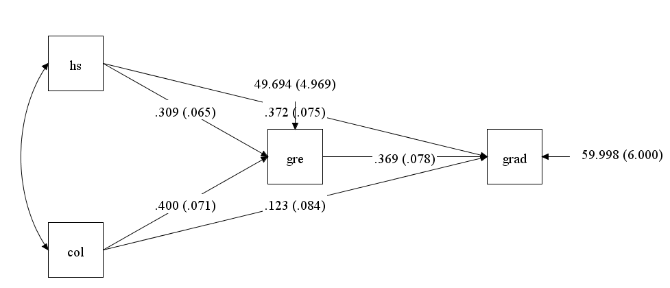
In the model command, the keyword on is used to indicate that the model regresses gre on hs and col, and grad on hs, col and gre. The
output command with the stdyx; option was included to obtain standardized regression coefficients and R-squared values. (The stdyx;
option produces coefficients standardized on both y and x, but other types of standardization are available and can be requested using the standardized; option.)
title: Path analysis -- just identified model

data:
file is path.dat;

variable:
names are hs gre col grad;

model:
gre on hs col;
grad on hs col gre;

output:
stdyx;
Here is the output from Mplus.
Path analysis -- just identified model

SUMMARY OF ANALYSIS

Number of groups                                                 1
Number of observations                                         200

Number of dependent variables                                    2
Number of independent variables                                  2
Number of continuous latent variables                            0

Observed dependent variables

  Continuous
   GRE         GRAD

Observed independent variables
   HS          COL


Estimator                                                       ML
Information matrix                                        OBSERVED
Maximum number of iterations                                  1000
Convergence criterion                                    0.500D-04
Maximum number of steepest descent iterations                   20

Input data file(s)
  D:/data/path.dat

Input data format  FREE

THE MODEL ESTIMATION TERMINATED NORMALLY

MODEL FIT INFORMATION

Number of Free Parameters                        9

Loglikelihood

          H0 Value                       -1367.594
          H1 Value                       -1367.594

Information Criteria

          Akaike (AIC)                    2753.189
          Bayesian (BIC)                  2782.874
          Sample-Size Adjusted BIC        2754.361
            (n* = (n + 2) / 24)

Chi-Square Test of Model Fit

          Value                              0.000
          Degrees of Freedom                     0
          P-Value                           0.0000

RMSEA (Root Mean Square Error Of Approximation)

          Estimate                           0.000
          90 Percent C.I.                    0.000  0.000
          Probability RMSEA <= .05           0.000

CFI/TLI

          CFI                                1.000
          TLI                                1.000

Chi-Square Test of Model Fit for the Baseline Model

          Value                            247.004
          Degrees of Freedom                     5
          P-Value                           0.0000

SRMR (Standardized Root Mean Square Residual)

          Value                              0.000

MODEL RESULTS

                                                    Two-Tailed
                    Estimate       S.E.  Est./S.E.    P-Value

 GRE      ON
    HS                 0.309      0.065      4.756      0.000
    COL                0.400      0.071      5.625      0.000

 GRAD     ON
    HS                 0.372      0.075      4.937      0.000
    COL                0.123      0.084      1.465      0.143
    GRE                0.369      0.078      4.754      0.000

 Intercepts
    GRE               15.534      2.995      5.186      0.000
    GRAD               6.971      3.506      1.989      0.047

 Residual Variances
    GRE               49.694      4.969     10.000      0.000
    GRAD              59.998      6.000     10.000      0.000

STANDARDIZED MODEL RESULTS


STDYX Standardization

                                                    Two-Tailed
                    Estimate       S.E.  Est./S.E.    P-Value

 GRE      ON
    HS                 0.335      0.068      4.887      0.000
    COL                0.396      0.068      5.859      0.000

 GRAD     ON
    HS                 0.356      0.070      5.073      0.000
    COL                0.108      0.073      1.467      0.142
    GRE                0.326      0.067      4.869      0.000

 Intercepts
    GRE                1.643      0.378      4.343      0.000
    GRAD               0.651      0.350      1.859      0.063

 Residual Variances
    GRE                0.556      0.052     10.611      0.000
    GRAD               0.523      0.051     10.240      0.000


R-SQUARE

    Observed                                        Two-Tailed
    Variable        Estimate       S.E.  Est./S.E.    P-Value

    GRE                0.444      0.052      8.477      0.000
    GRAD               0.477      0.051      9.333      0.000

QUALITY OF NUMERICAL RESULTS

     Condition Number for the Information Matrix              0.348E-04
       (ratio of smallest to largest eigenvalue)

DIAGRAM INFORMATION

  Use View Diagram under the Diagram menu in the Mplus Editor to view the diagram.
  If running Mplus from the Mplus Diagrammer, the diagram opens automatically.

  Diagram output
    d:datapath1.dgm
In the MODEL RESULTS section, the path coefficients (slopes) for the regression of gre on hs and col are shown, followed by those for the
regression grad on hs. Along with the unstandardized coefficients (in the column labeled Estimate), the standard errors (S.E), coefficients divided by the standard errors, and a p-values are shown. From this we see that hs and col significantly predict gre, and that gre
and hs (but not col) significantly predict grad. Additional parameters from the model are listed below the path coefficients. Note that
the regression intercepts are listed under the heading Intercepts rather than with the path coefficients. This is different from some general-purpose statistical packages where all of the coefficients (intercepts and slopes) are listed together. Because we requested standardized coefficients using the stdyx option of the output command, the standardized results are also included in the output (after the unstandardized results). Under the heading STDYX Standardization all of the model parameters are listed, standardized so that a one unit change represents a standard deviation change in the original variable (just as in a standardized regression model). As part of the standardized output, the r-squared values are presented under the heading R-SQUARE. Here the estimated r-squared value for each of the dependent variables in our model is given, along with standard errors and hypothesis tests.
2.0 Indirect and total effects
One of the appealing aspects of path models is the ability to assess indirect, as well as total effects (i.e., relationships among variables). Note that the total effect is the combination of the direct effect and indirect effects. In this example we will request the estimated indirect effect of hs on grad (through gre). Below is the diagram corresponding to this model with the desired indirect effect shown in blue. We can obtain the estimate of the indirect effect by adding the model indirect: command to our input file, and specifying grad ind hs;.
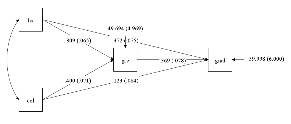
Here is the entire program. Notice that the model indirect has been added.
title:  Path analysis -- with indirect effects

data:
file is path.dat;

variable:
names are hs gre col grad;

model:
gre on hs col;
grad on hs col gre;

model indirect:
grad ind hs;

output:
stdyx;
The output for this model is shown below. The output is the same as the output from the previous example because we have estimated the same model; adding the indirect effects requests additional output from Mplus, but that does not change the model itself. The breakdown of the total, indirect, and direct effects appears below the MODEL RESULTS and STANDARDIZED MODEL RESULTS in a section labeled TOTAL, TOTAL INDIRECT, SPECIFIC INDIRECT, AND DIRECT EFFECTS. Because standardized coefficients were requested, the standardized total, indirect, and direct effects appear below the unstandardized effects.
Path analysis -- with indirect effects

SUMMARY OF ANALYSIS

Number of groups                                                 1
Number of observations                                         200

Number of dependent variables                                    2
Number of independent variables                                  2
Number of continuous latent variables                            0

Observed dependent variables

  Continuous
   GRE         GRAD

Observed independent variables
   HS          COL

Estimator                                                       ML
Information matrix                                        OBSERVED
Maximum number of iterations                                  1000
Convergence criterion                                    0.500D-04
Maximum number of steepest descent iterations                   20

Input data file(s)
    path.dat

Input data format  FREE

THE MODEL ESTIMATION TERMINATED NORMALLY

MODEL FIT INFORMATION

Number of Free Parameters                        9

Loglikelihood

          H0 Value                       -1367.594
          H1 Value                       -1367.594

Information Criteria

          Akaike (AIC)                    2753.189
          Bayesian (BIC)                  2782.874
          Sample-Size Adjusted BIC        2754.361
            (n* = (n + 2) / 24)

Chi-Square Test of Model Fit

          Value                              0.000
          Degrees of Freedom                     0
          P-Value                           0.0000

RMSEA (Root Mean Square Error Of Approximation)

          Estimate                           0.000
          90 Percent C.I.                    0.000  0.000
          Probability RMSEA <= .05           0.000

CFI/TLI

          CFI                                1.000
          TLI                                1.000

Chi-Square Test of Model Fit for the Baseline Model

          Value                            247.004
          Degrees of Freedom                     5
          P-Value                           0.0000

SRMR (Standardized Root Mean Square Residual)

          Value                              0.000

MODEL RESULTS

                                                    Two-Tailed
                    Estimate       S.E.  Est./S.E.    P-Value

 GRE      ON
    HS                 0.309      0.065      4.756      0.000
    COL                0.400      0.071      5.625      0.000

 GRAD     ON
    HS                 0.372      0.075      4.937      0.000
    COL                0.123      0.084      1.465      0.143
    GRE                0.369      0.078      4.754      0.000

 Intercepts
    GRE               15.534      2.995      5.186      0.000
    GRAD               6.971      3.506      1.989      0.047

 Residual Variances
    GRE               49.694      4.969     10.000      0.000
    GRAD              59.998      6.000     10.000      0.000

STANDARDIZED MODEL RESULTS

STDYX Standardization

                                                    Two-Tailed
                    Estimate       S.E.  Est./S.E.    P-Value

 GRE      ON
    HS                 0.335      0.068      4.887      0.000
    COL                0.396      0.068      5.859      0.000

 GRAD     ON
    HS                 0.356      0.070      5.073      0.000
    COL                0.108      0.073      1.467      0.142
    GRE                0.326      0.067      4.869      0.000

 Intercepts
    GRE                1.643      0.378      4.343      0.000
    GRAD               0.651      0.350      1.859      0.063

 Residual Variances
    GRE                0.556      0.052     10.611      0.000
    GRAD               0.523      0.051     10.240      0.000

R-SQUARE

    Observed                                        Two-Tailed
    Variable        Estimate       S.E.  Est./S.E.    P-Value

    GRE                0.444      0.052      8.477      0.000
    GRAD               0.477      0.051      9.333      0.000

QUALITY OF NUMERICAL RESULTS

     Condition Number for the Information Matrix              0.348E-04
       (ratio of smallest to largest eigenvalue)


TOTAL, TOTAL INDIRECT, SPECIFIC INDIRECT, AND DIRECT EFFECTS


                                                    Two-Tailed
                    Estimate       S.E.  Est./S.E.    P-Value

Effects from HS to GRAD

  Total                0.487      0.075      6.453      0.000
  Total indirect       0.114      0.034      3.362      0.001

  Specific indirect

    GRAD
    GRE
    HS                 0.114      0.034      3.362      0.001

  Direct
    GRAD
    HS                 0.372      0.075      4.937      0.000

STANDARDIZED TOTAL, TOTAL INDIRECT, SPECIFIC INDIRECT, AND DIRECT EFFECTS

STDYX Standardization

                                                    Two-Tailed
                    Estimate       S.E.  Est./S.E.    P-Value

Effects from HS to GRAD

  Total                0.465      0.068      6.858      0.000
  Total indirect       0.109      0.032      3.455      0.001

  Specific indirect

    GRAD
    GRE
    HS                 0.109      0.032      3.455      0.001

  Direct
    GRAD
    HS                 0.356      0.070      5.073      0.000

DIAGRAM INFORMATION

  Use View Diagram under the Diagram menu in the Mplus Editor to view the diagram.
  If running Mplus from the Mplus Diagrammer, the diagram opens automatically.

  Diagram output
    c:\temp\path2.dgm
Under Specific indirect, the effect labeled GRAD GRE HS (note that each appears on its own line and the final outcome is listed first), gives the estimated coefficient for the indirect effect of hs on grad, through GRE . The coefficient labeled Direct is the direct effect of hs on grad. We can say that part of the total effect of hs on grad is mediated by gre scores, but the significant direct path from hs to grad suggests only partial mediation.
3.0 Specific indirect effects
The above example was overly simple since there was only one indirect effect. Often models will have multiple indirect effects. In this example we place a directional path (i.e., regression) from hs to col, creating a model with multiple possible indirect effects. The diagram below shows the model.
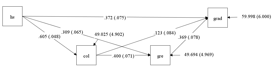
There are several ways to request calculation of indirect effects. The first, shown in the previous example (i.e., grad ind hs;) requests all indirect paths from hs to grad. We can also use ind to request a specific indirect path. For example, below we use grad ind col hs; to specify that we want to estimate the indirect effect from hs to col to grad. Finally, we can use via to request all indirect effects that go through a third variable. In the example below, we use grad via gre hs; to request all indirect paths from hs to grad that involve gre. This includes hs to gre to grad and hs to col to gre to grad.
title: Multiple indirect paths

data:
file is path.dat;

variable:
names are hs gre col grad;

model:
gre on col hs;
grad on hs col gre;
col on hs;

model indirect:
grad ind col hs;
grad via gre hs;

output: stdyx;
The abridged output is shown below. Note that the output for this model is similar in structure to the output from earlier models, except for the addition of the section showing the indirect effects.
<output omitted>
TOTAL, TOTAL INDIRECT, SPECIFIC INDIRECT, AND DIRECT EFFECTS


                                                    Two-Tailed
                    Estimate       S.E.  Est./S.E.    P-Value

Effects from HS to GRAD

  Indirect             0.075      0.051      1.455      0.146

Effects from HS to GRAD via GRE

  Sum of indirect      0.204      0.047      4.333      0.000

  Specific indirect
    GRAD
    GRE
    HS                 0.114      0.034      3.362      0.001

    GRAD
    GRE
    COL
    HS                 0.090      0.026      3.487      0.000

STANDARDIZED TOTAL, TOTAL INDIRECT, SPECIFIC INDIRECT, AND DIRECT EFFECTS

STDYX Standardization

                                                    Two-Tailed
                    Estimate       S.E.  Est./S.E.    P-Value

Effects from HS to GRAD

  Indirect             0.071      0.049      1.460      0.144

Effects from HS to GRAD via GRE

  Sum of indirect      0.195      0.043      4.533      0.000

  Specific indirect
    GRAD
    GRE
    HS                 0.109      0.032      3.455      0.001

    GRAD
    GRE
    COL
    HS                 0.086      0.024      3.587      0.000
The first set of indirect effects (labeled Effects from HS to GRAD) gives the indirect effect of hs on grad through col. Although we estimated a direct effect of hs on grad in the model, this is not shown in this portion of the output (it is shown above), because we requested the specific indirect effect. The second set of indirect effects (labeled Effects from HS to GRAD via GRE) shows all possible indirect effects from hs to grad that include GRE. In this example, there are two such effects. This portion of the output shows that hs has a significant indirect effect on grad, overall (Sum of indirect), as well as the two specific indirect effects, that is through gre, as well as through col and gre. Note that this output does not include the total effect of grad on hs; for this output we would simply specify grad ind hs; as we did in the previous model.