Mplus version 8 was used for these examples. All the files for this portion of this seminar can be downloaded here.
In other sections we have shown how to estimate two types of measurement models, confirmatory factor models and mixture models (e.g., latent class analysis). We have also shown how to estimate a path model, where relationships among observed variables are modeled. Structural equation models combine the two, using regression paths to estimate a model with a specific set of relationships among latent variables. Structural equation models typically impose restrictions on the relationships between the latent variables, that is, only a subset of the possible paths between the latent variables are included. The dataset to be used in the following examples is worland.dat.
1.0 A structural equation model
The following model continues from the example introduced in the confirmatory factor analysis page. The diagram below shows the model to be tested. Unlike a confirmatory factor analysis (CFA) model, where all of the latent variables are allowed to covary, this model specifies a set of relationships among the latent variables. Some of these relationships are directional (i.e., regression paths), and some are not (i.e., covariances). The model in our example also specifies that any covariance between cognitive and adjust is entirely through their relationships with other variables in the model.
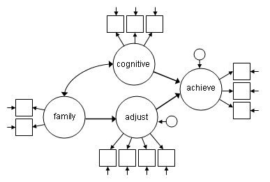
On the first four statements in model command block, we use the keyword by to define the four latent variables as we did in the CFA. Below those four statements, the keyword on is used to specify that we want to predict achieve using cognitive and adjust (i.e., achieve on cog adjust;). The model also predicts adjust using family (adjust on family;). Notice that the model command block does not include a covariance between family and cognitive (i.e., family with cog;). We could include this command, but it is not necessary, as Mplus will include this covariance by default.
title: A structural equation model

data:
      file is worland.dat;

variable:
      names are ppsych ses verbal vissp mem read arith spell motiv extra harm stabi;

model:
      family by ppsych ses;
      cog by verbal vissp mem;
      achieve by read arith spell;
      adjust by motiv extra harm stabi;
      achieve on cog adjust;
      adjust on family;
The abridged output for the above model is shown below.
A structural equation model

SUMMARY OF ANALYSIS

Number of groups                                                 1
Number of observations                                         500

Number of dependent variables                                   12
Number of independent variables                                  0
Number of continuous latent variables                            4

Observed dependent variables

  Continuous
   PPSYCH      SES         VERBAL      VISSP       MEM         READ
   ARITH       SPELL       MOTIV       EXTRA       HARM        STABI

Continuous latent variables
   FAMILY      COG         ACHIEVE     ADJUST


Estimator                                                       ML
Information matrix                                        OBSERVED
Maximum number of iterations                                  1000
Convergence criterion                                    0.500D-04
Maximum number of steepest descent iterations                   20

Input data file(s)
  worland.dat

Input data format  FREE

THE MODEL ESTIMATION TERMINATED NORMALLY

MODEL FIT INFORMATION

Number of Free Parameters                       40

Loglikelihood

          H0 Value                       -6762.779
          H1 Value                       -6445.272

Information Criteria

          Akaike (AIC)                   13605.559
          Bayesian (BIC)                 13774.143
          Sample-Size Adjusted BIC       13647.180
            (n* = (n + 2) / 24)

Chi-Square Test of Model Fit

          Value                            635.015
          Degrees of Freedom                    50
          P-Value                           0.0000

RMSEA (Root Mean Square Error Of Approximation)

          Estimate                           0.153
          90 Percent C.I.                    0.142  0.164
          Probability RMSEA <= .05           0.000

CFI/TLI

          CFI                                0.856
          TLI                                0.810

Chi-Square Test of Model Fit for the Baseline Model

          Value                           4124.707
          Degrees of Freedom                    66
          P-Value                           0.0000

SRMR (Standardized Root Mean Square Residual)

          Value                              0.067

MODEL RESULTS

                                                    Two-Tailed
                    Estimate       S.E.  Est./S.E.    P-Value

 FAMILY   BY
    PPSYCH             1.000      0.000    999.000    999.000
    SES               -1.093      0.121     -9.055      0.000

 COG      BY
    VERBAL             1.000      0.000    999.000    999.000
    VISSP              0.844      0.045     18.772      0.000
    MEM                0.969      0.044     21.797      0.000

 ACHIEVE  BY
    READ               1.000      0.000    999.000    999.000
    ARITH              0.836      0.034     24.715      0.000
    SPELL              0.951      0.027     35.681      0.000

 ADJUST   BY
    MOTIV              1.000      0.000    999.000    999.000
    EXTRA              0.232      0.049      4.749      0.000
    HARM               0.867      0.043     20.248      0.000
    STABI              0.669      0.045     14.697      0.000

 ACHIEVE  ON
    COG                0.892      0.050     17.692      0.000
    ADJUST             0.139      0.040      3.485      0.000

 ADJUST   ON
    FAMILY            -1.183      0.135     -8.783      0.000

 COG      WITH
    FAMILY            -0.412      0.046     -9.019      0.000

 Intercepts
    PPSYCH             0.000      0.045      0.000      1.000
    SES                0.000      0.045      0.000      1.000
    VERBAL             0.000      0.045      0.000      1.000
    VISSP              0.000      0.045      0.000      1.000
    MEM                0.000      0.045      0.000      1.000
    READ               0.000      0.045      0.000      1.000
    ARITH              0.000      0.045      0.000      1.000
    SPELL              0.000      0.045      0.000      1.000
    MOTIV              0.000      0.045      0.000      1.000
    EXTRA              0.000      0.045      0.000      1.000
    HARM               0.000      0.045      0.000      1.000
    STABI              0.000      0.045      0.000      1.000

 Variances
    FAMILY             0.252      0.049      5.119      0.000
    COG                0.745      0.064     11.668      0.000

 Residual Variances
    PPSYCH             0.746      0.054     13.883      0.000
    SES                0.697      0.052     13.467      0.000
    VERBAL             0.253      0.025     10.255      0.000
    VISSP              0.467      0.034     13.626      0.000
    MEM                0.299      0.027     11.143      0.000
    READ               0.096      0.014      6.855      0.000
    ARITH              0.367      0.027     13.676      0.000
    SPELL              0.183      0.016     11.458      0.000
    MOTIV              0.107      0.032      3.346      0.001
    EXTRA              0.950      0.061     15.700      0.000
    HARM               0.328      0.033     10.039      0.000
    STABI              0.600      0.042     14.252      0.000
    ACHIEVE            0.170      0.022      7.845      0.000
    ADJUST             0.539      0.053     10.170      0.000

QUALITY OF NUMERICAL RESULTS

     Condition Number for the Information Matrix              0.316E-02
       (ratio of smallest to largest eigenvalue)

DIAGRAM INFORMATION

  Use View Diagram under the Diagram menu in the Mplus Editor to view the diagram.
  If running Mplus from the Mplus Diagrammer, the diagram opens automatically.

  Diagram output
    c:\temp\01-sem.dgm
In the MODEL RESULTS section of the above output, we first see the measurement portion of the model where the four latent variables are defined. The next section shows the structural portion of the model predicting achieve (ACHIEVE ON) and adjust (ADJUST ON). The coefficients shown under ACHIEVE ON are the coefficients from the latent variable achieve regressed on the latent variables cog and adjust, and they can be interpreted as regression coefficients. The standard errors, the ratio of the coefficient to its standard error (i.e., a t- or z-value), and a p-value are also given for each structural coefficient. Below the regression results is the estimate of the covariance between the exogenous latent variables cog and family. The rest of the output is similar to the output for the measurement model except that, rather than having a variance (listed under Variances), achieve and adjust now have residual variances (listed under Residual Variances) because they are being predicted by other variables in the model.
2.0 Including an observed variable in the structural model
It is possible to include observed variables in the structural portion of the model. In the earlier models, the observed variables ses and ppsych were used to estimate the latent variable family. In the current model, the variable ses is removed from the model entirely, and the variable ppsych remains as a single observed variable predicting the latent variable adjust. The diagram below shows this model.
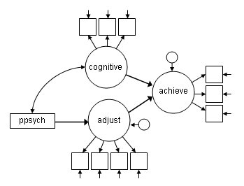
Removing ses from the model and including ppsych as an observed variable requires a few relatively small changes to the model. The first is that we have added the usevariables statement in the variables command block. By default Mplus includes all variables in the dataset in the model. (Note that the names statement tells Mplus the number, names, and order of the variables in the dataset, so we do not want to make any changes to it.) The usevariables statement allows us to tell Mplus that we want to use a subset of the variables in our file. Since we only want to exclude ses, the usevariables statement is followed by the names of all the variables in our dataset except ses. The second change is that we have removed the line in the model command block that was used to define the latent variable family because we no longer want to estimate that latent variable. The final change is that we now use ppsych to predict adjust (i.e., adjust on ppsych;). The final statement, ppsych with cog; allows ppsych and cog to covary.
title: Adding an observed variable in the structural model

data:
     file is worland.dat;

variable:
      names are ppsych ses verbal vissp mem read arith spell motiv extra harm stabi;
      usevariables are ppsych verbal vissp mem read arith spell motiv extra harm stabi;

model:
      cog by verbal vissp mem;
      achieve by read arith spell;
      adjust by motiv extra harm stabi;
      achieve on cog adjust;
      adjust on ppsych;
      ppsych with cog;
The output for this model is shown below.
INPUT READING TERMINATED NORMALLY

Adding an observed variable in the structural model;

SUMMARY OF ANALYSIS

Number of groups                                                 1
Number of observations                                         500

Number of dependent variables                                   10
Number of independent variables                                  1
Number of continuous latent variables                            3

Observed dependent variables

  Continuous
   VERBAL      VISSP       MEM         READ        ARITH       SPELL
   MOTIV       EXTRA       HARM        STABI

Observed independent variables
   PPSYCH

Continuous latent variables
   COG         ACHIEVE     ADJUST


Estimator                                                       ML
Information matrix                                        OBSERVED
Maximum number of iterations                                  1000
Convergence criterion                                    0.500D-04
Maximum number of steepest descent iterations                   20

Input data file(s)
  worland.dat

Input data format  FREE

THE MODEL ESTIMATION TERMINATED NORMALLY

MODEL FIT INFORMATION

Number of Free Parameters                       36

Loglikelihood

          H0 Value                       -6198.772
          H1 Value                       -5834.042

Information Criteria

          Akaike (AIC)                   12469.544
          Bayesian (BIC)                 12621.270
          Sample-Size Adjusted BIC       12507.004
            (n* = (n + 2) / 24)

Chi-Square Test of Model Fit

          Value                            729.459
          Degrees of Freedom                    41
          P-Value                           0.0000

RMSEA (Root Mean Square Error Of Approximation)

          Estimate                           0.183
          90 Percent C.I.                    0.172  0.195
          Probability RMSEA <= .05           0.000

CFI/TLI

          CFI                                0.822
          TLI                                0.762

Chi-Square Test of Model Fit for the Baseline Model

          Value                           3929.228
          Degrees of Freedom                    55
          P-Value                           0.0000

SRMR (Standardized Root Mean Square Residual)

          Value                              0.153

MODEL RESULTS

                                                    Two-Tailed
                    Estimate       S.E.  Est./S.E.    P-Value

 COG      BY
    VERBAL             1.000      0.000    999.000    999.000
    VISSP              0.865      0.046     18.821      0.000
    MEM                0.963      0.046     20.863      0.000

 ACHIEVE  BY
    READ               1.000      0.000    999.000    999.000
    ARITH              0.836      0.034     24.686      0.000
    SPELL              0.952      0.027     35.669      0.000

 ADJUST   BY
    MOTIV              1.000      0.000    999.000    999.000
    EXTRA              0.222      0.051      4.393      0.000
    HARM               0.898      0.052     17.388      0.000
    STABI              0.688      0.049     13.928      0.000

 ACHIEVE  ON
    COG                0.859      0.046     18.690      0.000
    ADJUST             0.216      0.035      6.116      0.000

 ADJUST   ON
    PPSYCH            -0.254      0.042     -6.008      0.000

 PPSYCH   WITH
    COG               -0.396      0.046     -8.667      0.000

 Means
    PPSYCH             0.000      0.045      0.000      1.000

 Intercepts
    VERBAL             0.000      0.045      0.000      1.000
    VISSP              0.000      0.045      0.000      1.000
    MEM                0.000      0.045      0.000      1.000
    READ               0.000      0.041      0.000      1.000
    ARITH              0.000      0.042      0.000      1.000
    SPELL              0.000      0.042      0.000      1.000
    MOTIV              0.000      0.043      0.000      1.000
    EXTRA              0.000      0.045      0.000      1.000
    HARM               0.000      0.043      0.000      1.000
    STABI              0.000      0.044      0.000      1.000

 Variances
    PPSYCH             0.998      0.063     15.811      0.000
    COG                0.738      0.064     11.488      0.000

 Residual Variances
    VERBAL             0.260      0.026      9.913      0.000
    VISSP              0.445      0.034     13.158      0.000
    MEM                0.313      0.029     10.965      0.000
    READ               0.097      0.014      6.853      0.000
    ARITH              0.368      0.027     13.703      0.000
    SPELL              0.181      0.016     11.385      0.000
    MOTIV              0.136      0.041      3.322      0.001
    EXTRA              0.955      0.061     15.671      0.000
    HARM               0.303      0.039      7.826      0.000
    STABI              0.589      0.043     13.851      0.000
    ACHIEVE            0.170      0.022      7.740      0.000
    ADJUST             0.798      0.070     11.388      0.000

QUALITY OF NUMERICAL RESULTS

     Condition Number for the Information Matrix              0.145E-01
       (ratio of smallest to largest eigenvalue)

DIAGRAM INFORMATION

  Use View Diagram under the Diagram menu in the Mplus Editor to view the diagram.
  If running Mplus from the Mplus Diagrammer, the diagram opens automatically.

  Diagram output
    c:\temp\02-sem.dgm
The MODEL RESULTS section begins with the three (instead of four) latent variables in the model. In the structural (on) portion of the output, the coefficient for adjust regressed on ppsych is presented in the output the same way the coefficients for the latent predictor variables are reported. Below that, the covariance between ppsych and cog is shown under the heading PPSYCH WITH. The rest of the output is similar to the previous models.
Additional output
Above we have shown only the default output for each model, but a range of additional output can be requested using the Output command block. Below we show a few commonly used output options.
3.0 Sample statistics
The input below is the same as the input for our first model except for the addition of the Output command block. We use the sampstat; option to request that sample statistics (observed variable means, covariances and correlations) be included in the output.
title: Adding output

data:
     file is worland.dat;

variable:
     names are
     ppsych ses verbal vissp mem read arith spell motiv extra harm stabi;

model:
     family by ppsych ses;
     cog by verbal vissp  mem;
     achieve by read arith spell;
     adjust by motiv extra harm stabi;
     achieve on cog adjust;
     adjust on family;
output: sampstat;
Below we show the additional output provided by the sampstat; option (all other output has been omitted to save space). The “sample statistics” section shown below appears towards the top of the output file, after the “summary of analysis” and before the “tests of model fit”.
SAMPLE STATISTICS

     SAMPLE STATISTICS


           Means
              PPSYCH        SES           VERBAL        VISSP         MEM
              ________      ________      ________      ________      ________
      1         0.000         0.000         0.000         0.000         0.000


           Means
              READ          ARITH         SPELL         MOTIV         EXTRA
              ________      ________      ________      ________      ________
      1         0.000         0.000         0.000         0.000         0.000


           Means
              HARM          STABI
              ________      ________
      1         0.000         0.000


           Covariances
              PPSYCH        SES           VERBAL        VISSP         MEM
              ________      ________      ________      ________      ________
 PPSYCH         0.998
 SES           -0.419         0.998
 VERBAL        -0.429         0.499         0.998
 VISSP         -0.399         0.399         0.659         0.998
 MEM           -0.349         0.379         0.669         0.659         0.998
 READ          -0.389         0.429         0.778         0.559         0.729
 ARITH         -0.240         0.369         0.689         0.489         0.699
 SPELL         -0.309         0.329         0.629         0.479         0.719
 MOTIV         -0.250         0.249         0.489         0.319         0.579
 EXTRA         -0.140         0.170         0.180         0.090         0.170
 HARM          -0.249         0.259         0.419         0.249         0.459
 STABI         -0.160         0.180         0.329         0.269         0.349


           Covariances
              READ          ARITH         SPELL         MOTIV         EXTRA
              ________      ________      ________      ________      ________
 READ           0.998
 ARITH          0.729         0.998
 SPELL          0.868         0.719         0.998
 MOTIV          0.529         0.599         0.589         0.998
 EXTRA          0.140         0.150         0.150         0.249         0.998
 HARM           0.419         0.439         0.449         0.768         0.190
 STABI          0.359         0.379         0.379         0.589        -0.289


           Covariances
              HARM          STABI
              ________      ________
 HARM           0.998
 STABI          0.579         0.998


           Correlations
              PPSYCH        SES           VERBAL        VISSP         MEM
              ________      ________      ________      ________      ________
 PPSYCH         1.000
 SES           -0.420         1.000
 VERBAL        -0.430         0.500         1.000
 VISSP         -0.400         0.400         0.660         1.000
 MEM           -0.350         0.380         0.670         0.660         1.000
 READ          -0.390         0.430         0.780         0.560         0.730
 ARITH         -0.240         0.370         0.690         0.490         0.700
 SPELL         -0.310         0.330         0.630         0.480         0.720
 MOTIV         -0.250         0.250         0.490         0.320         0.580
 EXTRA         -0.140         0.170         0.180         0.090         0.170
 HARM          -0.250         0.260         0.420         0.250         0.460
 STABI         -0.160         0.180         0.330         0.270         0.350


           Correlations
              READ          ARITH         SPELL         MOTIV         EXTRA
              ________      ________      ________      ________      ________
 READ           1.000
 ARITH          0.730         1.000
 SPELL          0.870         0.720         1.000
 MOTIV          0.530         0.600         0.590         1.000
 EXTRA          0.140         0.150         0.150         0.250         1.000
 HARM           0.420         0.440         0.450         0.770         0.190
 STABI          0.360         0.380         0.380         0.590        -0.290


           Correlations
              HARM          STABI
              ________      ________
 HARM           1.000
 STABI          0.580         1.000


UNIVARIATE SAMPLE STATISTICS

     UNIVARIATE HIGHER-ORDER MOMENT DESCRIPTIVE STATISTICS

         Variable/         Mean/     Skewness/   Minimum/ % with                Percentiles
        Sample Size      Variance    Kurtosis    Maximum  Min/Max      20%/60%    40%/80%    Median

     PPSYCH                0.000       0.094      -3.109    0.20%      -0.829     -0.272     -0.054
             500.000       0.998      -0.054       3.328    0.20%       0.208      0.809
     SES                   0.000       0.068      -3.214    0.20%      -0.834     -0.262     -0.031
             500.000       0.998      -0.037       2.910    0.20%       0.234      0.842
     VERBAL                0.000      -0.226      -3.526    0.20%      -0.788     -0.222     -0.018
             500.000       0.998       0.524       3.170    0.20%       0.241      0.849
     VISSP                 0.000      -0.091      -3.761    0.20%      -0.793     -0.243      0.005
             500.000       0.998       0.377       2.766    0.20%       0.231      0.796
     MEM                   0.000      -0.040      -3.123    0.20%      -0.777     -0.249     -0.050
             500.000       0.998       0.034       2.518    0.20%       0.210      0.865
     READ                  0.000      -0.112      -3.284    0.20%      -0.859     -0.209     -0.004
             500.000       0.998       0.103       2.761    0.20%       0.267      0.820
     ARITH                 0.000      -0.017      -2.670    0.20%      -0.825     -0.189      0.013
             500.000       0.998       0.051       3.305    0.20%       0.246      0.800
     SPELL                 0.000      -0.123      -3.136    0.20%      -0.808     -0.206     -0.001
             500.000       0.998      -0.007       2.693    0.20%       0.272      0.815
     MOTIV                 0.000      -0.102      -3.397    0.20%      -0.862     -0.190      0.032
             500.000       0.998      -0.152       2.647    0.20%       0.263      0.867
     EXTRA                 0.000       0.117      -3.222    0.20%      -0.799     -0.324     -0.105
             500.000       0.998      -0.012       3.137    0.20%       0.178      0.893
     HARM                  0.000      -0.149      -3.298    0.20%      -0.806     -0.234      0.001
             500.000       0.998       0.330       3.116    0.20%       0.264      0.853
     STABI                 0.000      -0.061      -2.592    0.20%      -0.861     -0.230      0.030
             500.000       0.998      -0.384       2.963    0.20%       0.263      0.868
4.0 Standardized coefficients
Standardized coefficients, and, with some models, R2, can be obtained using the standardized option of the output command block. Mplus actually produces three forms of standardized coefficients, labeled stdyx, stdy and std. Using the standardized option requests all three, using these names as options one allows the user to request that only one (or two) sets of standardized estimates be printed. Below the output command block is shown; the input file is otherwise unchanged.
output:
  standardized;
or
output: stdyx;
The full code is listed here:
title: Getting standardized coefficients;

data: file is worland.dat;

variable:
 names are
     ppsych ses verbal vissp mem read arith spell motiv extra harm stabi;

model:
     family by ppsych ses;
     cog by verbal vissp  mem;
     achieve by read arith spell;
     adjust by motiv extra harm stabi;
     achieve on cog adjust;
     adjust on family;
output: standardized;
The abridged output (using standardized;) is shown below.
<output omitted>
STANDARDIZED MODEL RESULTS
STDYX Standardization
Two-Tailed
Estimate S.E. Est./S.E. P-Value
FAMILY BY
PPSYCH 0.502 0.042 11.913 0.000
SES -0.549 0.040 -13.780 0.000
COG BY
VERBAL 0.864 0.016 55.058 0.000
VISSP 0.729 0.024 30.279 0.000
MEM 0.837 0.018 47.624 0.000
ACHIEVE BY
READ 0.950 0.008 119.258 0.000
ARITH 0.795 0.019 42.875 0.000
SPELL 0.904 0.010 88.543 0.000
ADJUST BY
MOTIV 0.945 0.017 54.666 0.000
EXTRA 0.219 0.046 4.798 0.000
HARM 0.819 0.021 38.479 0.000
STABI 0.632 0.031 20.699 0.000
ACHIEVE ON
COG 0.811 0.032 25.571 0.000
ADJUST 0.138 0.040 3.454 0.001
ADJUST ON
FAMILY -0.629 0.036 -17.328 0.000
COG WITH
FAMILY -0.950 0.035 -26.824 0.000
Intercepts
PPSYCH 0.000 0.045 0.000 1.000
SES 0.000 0.045 0.000 1.000
VERBAL 0.000 0.045 0.000 1.000
VISSP 0.000 0.045 0.000 1.000
MEM 0.000 0.045 0.000 1.000
READ 0.000 0.045 0.000 1.000
ARITH 0.000 0.045 0.000 1.000
SPELL 0.000 0.045 0.000 1.000
MOTIV 0.000 0.045 0.000 1.000
EXTRA 0.000 0.045 0.000 1.000
HARM 0.000 0.045 0.000 1.000
STABI 0.000 0.045 0.000 1.000
Variances
FAMILY 1.000 0.000 999.000 999.000
COG 1.000 0.000 999.000 999.000
Residual Variances
PPSYCH 0.748 0.042 17.663 0.000
SES 0.698 0.044 15.959 0.000
VERBAL 0.253 0.027 9.331 0.000
VISSP 0.468 0.035 13.312 0.000
MEM 0.299 0.029 10.175 0.000
READ 0.097 0.015 6.386 0.000
ARITH 0.368 0.029 12.509 0.000
SPELL 0.183 0.018 9.929 0.000
MOTIV 0.107 0.033 3.288 0.001
EXTRA 0.952 0.020 47.670 0.000
HARM 0.328 0.035 9.410 0.000
STABI 0.601 0.039 15.588 0.000
ACHIEVE 0.189 0.025 7.645 0.000
ADJUST 0.605 0.046 13.249 0.000
STDY Standardization
Two-Tailed
Estimate S.E. Est./S.E. P-Value
FAMILY BY
PPSYCH 0.502 0.042 11.913 0.000
SES -0.549 0.040 -13.780 0.000
COG BY
VERBAL 0.864 0.016 55.058 0.000
VISSP 0.729 0.024 30.279 0.000
MEM 0.837 0.018 47.624 0.000
ACHIEVE BY
READ 0.950 0.008 119.258 0.000
ARITH 0.795 0.019 42.875 0.000
SPELL 0.904 0.010 88.543 0.000
ADJUST BY
MOTIV 0.945 0.017 54.666 0.000
EXTRA 0.219 0.046 4.798 0.000
HARM 0.819 0.021 38.479 0.000
STABI 0.632 0.031 20.699 0.000
ACHIEVE ON
COG 0.811 0.032 25.571 0.000
ADJUST 0.138 0.040 3.454 0.001
ADJUST ON
FAMILY -0.629 0.036 -17.328 0.000
COG WITH
FAMILY -0.950 0.035 -26.824 0.000
Intercepts
PPSYCH 0.000 0.045 0.000 1.000
SES 0.000 0.045 0.000 1.000
VERBAL 0.000 0.045 0.000 1.000
VISSP 0.000 0.045 0.000 1.000
MEM 0.000 0.045 0.000 1.000
READ 0.000 0.045 0.000 1.000
ARITH 0.000 0.045 0.000 1.000
SPELL 0.000 0.045 0.000 1.000
MOTIV 0.000 0.045 0.000 1.000
EXTRA 0.000 0.045 0.000 1.000
HARM 0.000 0.045 0.000 1.000
STABI 0.000 0.045 0.000 1.000
Variances
FAMILY 1.000 0.000 999.000 999.000
COG 1.000 0.000 999.000 999.000
Residual Variances
PPSYCH 0.748 0.042 17.663 0.000
SES 0.698 0.044 15.959 0.000
VERBAL 0.253 0.027 9.331 0.000
VISSP 0.468 0.035 13.312 0.000
MEM 0.299 0.029 10.175 0.000
READ 0.097 0.015 6.386 0.000
ARITH 0.368 0.029 12.509 0.000
SPELL 0.183 0.018 9.929 0.000
MOTIV 0.107 0.033 3.288 0.001
EXTRA 0.952 0.020 47.670 0.000
HARM 0.328 0.035 9.410 0.000
STABI 0.601 0.039 15.588 0.000
ACHIEVE 0.189 0.025 7.645 0.000
ADJUST 0.605 0.046 13.249 0.000
STD Standardization
Two-Tailed
Estimate S.E. Est./S.E. P-Value
FAMILY BY
PPSYCH 0.502 0.049 10.237 0.000
SES -0.549 0.048 -11.423 0.000
COG BY
VERBAL 0.863 0.037 23.337 0.000
VISSP 0.729 0.040 18.177 0.000
MEM 0.836 0.038 22.142 0.000
ACHIEVE BY
READ 0.949 0.034 28.126 0.000
ARITH 0.793 0.038 20.949 0.000
SPELL 0.902 0.035 25.881 0.000
ADJUST BY
MOTIV 0.944 0.037 25.405 0.000
EXTRA 0.219 0.047 4.645 0.000
HARM 0.819 0.040 20.707 0.000
STABI 0.631 0.043 14.848 0.000
ACHIEVE ON
COG 0.811 0.032 25.571 0.000
ADJUST 0.138 0.040 3.454 0.001
ADJUST ON
FAMILY -0.629 0.036 -17.328 0.000
COG WITH
FAMILY -0.950 0.035 -26.824 0.000
Intercepts
PPSYCH 0.000 0.045 0.000 1.000
SES 0.000 0.045 0.000 1.000
VERBAL 0.000 0.045 0.000 1.000
VISSP 0.000 0.045 0.000 1.000
MEM 0.000 0.045 0.000 1.000
READ 0.000 0.045 0.000 1.000
ARITH 0.000 0.045 0.000 1.000
SPELL 0.000 0.045 0.000 1.000
MOTIV 0.000 0.045 0.000 1.000
EXTRA 0.000 0.045 0.000 1.000
HARM 0.000 0.045 0.000 1.000
STABI 0.000 0.045 0.000 1.000
Variances
FAMILY 1.000 0.000 999.000 999.000
COG 1.000 0.000 999.000 999.000
Residual Variances
PPSYCH 0.746 0.054 13.883 0.000
SES 0.697 0.052 13.467 0.000
VERBAL 0.253 0.025 10.255 0.000
VISSP 0.467 0.034 13.626 0.000
MEM 0.299 0.027 11.143 0.000
READ 0.096 0.014 6.855 0.000
ARITH 0.367 0.027 13.676 0.000
SPELL 0.183 0.016 11.458 0.000
MOTIV 0.107 0.032 3.346 0.001
EXTRA 0.950 0.061 15.700 0.000
HARM 0.328 0.033 10.039 0.000
STABI 0.600 0.042 14.252 0.000
ACHIEVE 0.189 0.025 7.645 0.000
ADJUST 0.605 0.046 13.249 0.000
R-SQUARE
Observed Two-Tailed
Variable Estimate S.E. Est./S.E. P-Value
PPSYCH 0.252 0.042 5.957 0.000
SES 0.302 0.044 6.890 0.000
VERBAL 0.747 0.027 27.529 0.000
VISSP 0.532 0.035 15.139 0.000
MEM 0.701 0.029 23.812 0.000
READ 0.903 0.015 59.629 0.000
ARITH 0.632 0.029 21.438 0.000
SPELL 0.817 0.018 44.272 0.000
MOTIV 0.893 0.033 27.333 0.000
EXTRA 0.048 0.020 2.399 0.016
HARM 0.672 0.035 19.239 0.000
STABI 0.399 0.039 10.350 0.000
Latent Two-Tailed
Variable Estimate S.E. Est./S.E. P-Value
ACHIEVE 0.811 0.025 32.837 0.000
ADJUST 0.395 0.046 8.664 0.000
QUALITY OF NUMERICAL RESULTS
Condition Number for the Information Matrix 0.316E-02
(ratio of smallest to largest eigenvalue)
DIAGRAM INFORMATION
Use View Diagram under the Diagram menu in the Mplus Editor to view the diagram.
If running Mplus from the Mplus Diagrammer, the diagram opens automatically.
Diagram output
c:\temp\04-sem.dgm
5.0 Modification indices
It is necessary for every model makes certain assumptions. One common assumption is that a parameter is equal to a given value, often 0 (e.g., there is no direct relationship between two variables). Modification indices can be used to help evaluate how reasonable these assumptions are by giving the researcher a sense of what happens when those assumptions are relaxed. Modification indices can be obtained using the modindices option of the output command. Below we show only the output command; the input file remains otherwise unchanged. By default Mplus prints only those parameters with an MI greater than or equal to 10. Other values can be requested by following the option name with a number in parentheses. For example, to get all parameters with an MI greater than or equal to 3.84, the option should read modindices(3.84);.
output:
  modindices;
The modification indices are printed at the bottom of the output. The abridged output is shown below.
<output omitted>

MODEL MODIFICATION INDICES

NOTE:  Modification indices for direct effects of observed dependent variables
regressed on covariates may not be included.  To include these, request
MODINDICES (ALL).

Minimum M.I. value for printing the modification index    10.000

                                   M.I.     E.P.C.  Std E.P.C.  StdYX E.P.C.

BY Statements

FAMILY   BY ARITH                 25.688    -0.950     -0.476       -0.477
FAMILY   BY SPELL                 55.852     1.362      0.683        0.685
COG      BY READ                  12.220     0.389      0.336        0.337
COG      BY ARITH                 25.970     0.557      0.481        0.482
COG      BY SPELL                 60.413    -0.816     -0.705       -0.706
ACHIEVE  BY PPSYCH                10.712     0.426      0.404        0.405
ACHIEVE  BY VISSP                 53.047    -0.863     -0.819       -0.820
ACHIEVE  BY MEM                   41.805     0.800      0.759        0.759
ADJUST   BY VISSP                 21.664    -0.230     -0.217       -0.217
ADJUST   BY MEM                   35.432     0.270      0.255        0.255
ADJUST   BY READ                  43.012    -0.225     -0.212       -0.213
ADJUST   BY ARITH                 30.444     0.236      0.223        0.223

ON/BY Statements

FAMILY   ON ACHIEVE  /
ACHIEVE  BY FAMILY                15.990     0.389      0.735        0.735
FAMILY   ON ADJUST   /
ADJUST   BY FAMILY                28.827     0.419      0.787        0.787
COG      ON ACHIEVE  /
ACHIEVE  BY COG                   16.637     0.715      0.785        0.785
COG      ON ADJUST   /
ADJUST   BY COG                   28.833     0.684      0.748        0.748
ACHIEVE  ON FAMILY   /
FAMILY   BY ACHIEVE               10.036     2.205      1.166        1.166
ADJUST   ON COG      /
COG      BY ADJUST                28.859     5.085      4.651        4.651
ADJUST   ON ACHIEVE  /
ACHIEVE  BY ADJUST                36.095     5.338      5.366        5.366

WITH Statements

SES      WITH PPSYCH              28.832    -0.208     -0.208       -0.289
VERBAL   WITH SES                 11.340     0.081      0.081        0.192
MEM      WITH SES                 10.444    -0.080     -0.080       -0.175
MEM      WITH VERBAL              65.436    -0.185     -0.185       -0.675
MEM      WITH VISSP               15.179     0.086      0.086        0.230
READ     WITH VERBAL              48.872     0.088      0.088        0.564
READ     WITH MEM                 17.206    -0.054     -0.054       -0.316
ARITH    WITH PPSYCH              16.777     0.103      0.103        0.197
ARITH    WITH MEM                 13.462     0.065      0.065        0.196
ARITH    WITH READ                35.994    -0.100     -0.100       -0.531
SPELL    WITH SES                 12.814    -0.068     -0.068       -0.190
SPELL    WITH VERBAL              60.339    -0.105     -0.105       -0.489
SPELL    WITH MEM                 26.201     0.072      0.072        0.307
SPELL    WITH READ                44.080     0.143      0.143        1.080
MOTIV    WITH SES                 10.622    -0.074     -0.074       -0.272
MOTIV    WITH MEM                 19.099     0.069      0.069        0.385
MOTIV    WITH READ                18.150    -0.048     -0.048       -0.475
MOTIV    WITH ARITH               24.267     0.078      0.078        0.395
MOTIV    WITH SPELL               12.809     0.044      0.044        0.317
EXTRA    WITH MOTIV               33.375     0.158      0.158        0.494
HARM     WITH MOTIV               11.324    -0.188     -0.188       -1.004
STABI    WITH EXTRA              171.608    -0.458     -0.458       -0.606
STABI    WITH HARM                20.923     0.132      0.132        0.298
ACHIEVE  WITH FAMILY              10.037     0.054      0.261        0.261
ACHIEVE  WITH COG                 10.037     0.098      0.275        0.275
ADJUST   WITH FAMILY              28.832     0.225      0.612        0.612
ADJUST   WITH COG                 28.834     0.369      0.582        0.582
ADJUST   WITH ACHIEVE             10.058     1.005      3.322        3.322


DIAGRAM INFORMATION

  Use View Diagram under the Diagram menu in the Mplus Editor to view the diagram.
  If running Mplus from the Mplus Diagrammer, the diagram opens automatically.

  Diagram output
    c:\temp\05-sem.dgm
Data source
The data for these examples is based on a correlation matrix published in Worland et. al., 1984. Although the correlation matrix would have been sufficient to specify these models, 500 cases were randomly drawn from the distribution described by the published correlation matrix. The models above do not necessarily match those specified in Worland et. al., 1984, they are intended as examples only.
Worland, Julien, David G. Weeks, Cynthia L. Janes, and Strock, Barbara D. (1984) Intelligence, classroom behavior, and academic achievement in children at high and low risk for psychopathology: A structural equation analysis. Journal of Abnormal Child Psychology Vol. 12, No. 3, pp. 437-454.