Supplemental notes to Applied Survival Analysis
Tests of Proportionality in SAS, STATA and SPLUS
When modeling a Cox proportional hazard model a key assumption is proportional hazards. There are a number of basic concepts for testing proportionality but the implementation of these concepts differ across statistical packages. The goal of this page is to illustrate how to test for proportionality in STATA, SAS and SPLUS using an example from Applied Survival Analysis by Hosmer and Lemeshow .
1. Kaplan-Meier Curves
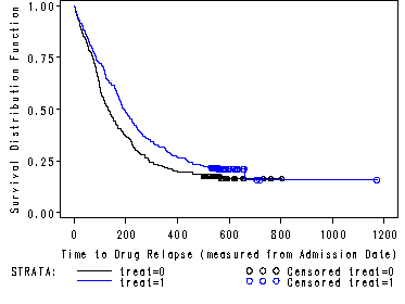
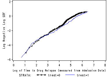
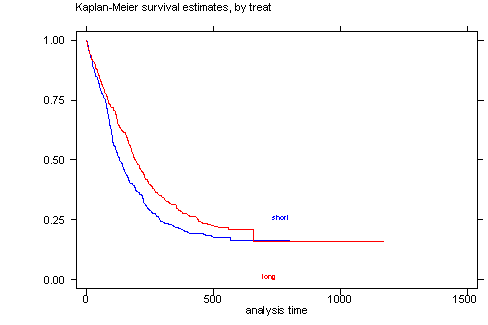
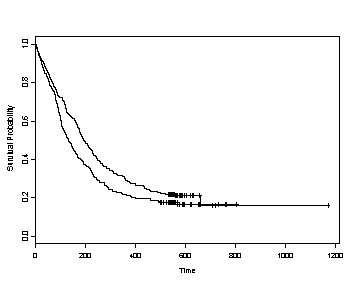
Works best for time fixed covariates with few levels. If the predictor satisfy the proportional hazard assumption then the graph of the survival function versus the survival time should results in a graph with parallel curves, similarly the graph of the log(-log(survival)) versus log of survival time graph should result in parallel lines if the predictor is proportional. This method does not work well for continuous predictor or categorical predictors that have many levels because the graph becomes to “cluttered”. Furthermore, the curves are sparse when there are fewer time points and it may be difficult to gage how close to parallel is close enough. Due to space limitations we will only show the graph for the predictor treat.
SAS It is very easy to create the graphs in SAS using proc lifetest. The plot option in the model statement lets you specify both the survival function versus time as well as the log(-log(survival) versus log(time).
proc lifetest data=uis plot=(s, lls) noprint;
  time time*censor(0);
  strata treat;
run;
STATA The sts graph command in STATA will generate the survival function versus time graph.
sts graph, by(treat)
SPLUS The plot function applied to a survfit object will generate a graph of the survival function versus the survival time.
plot(survfit(formula = Surv(time, censor)~ treat, data = uis, conf.type="none"),
     lty=0, xlab="Time", ylab="Survival Probability" )
2. Including Time Dependent Covariates in the Cox Model
Generate the time dependent covariates by creating interactions of the predictors and a function of survival time and include in the model. If any of the time dependent covariates are significant then those predictors are not proportional.
SAS In SAS it is possible to create all the time dependent variable inside proc phreg as demonstrated. Furthermore, by using the test statement is is possibly to test all the time dependent covariates all at once.
proc phreg data=uis;
  model time*censor(0) = age race treat site agesite aget racet treatt sitet;
  aget = age*log(time);
  racet = race*log(time);
  treatt = treat*log(time);
  sitet = site*log(time);
  proportionality_test: test aget, racet, treat, sitet;
run;
<output omitted>

               Analysis of Maximum Likelihood Estimates

                   Parameter      Standard
Variable    DF      Estimate         Error    Chi-Square    Pr > ChiSq
age          1      -0.02932       0.03336        0.7729        0.3793
race         1      -0.99201       0.53252        3.4702        0.0625
treat        1      -0.52086       0.40742        1.6344        0.2011
site         1      -1.48805       0.67291        4.8901        0.0270
agesite      1       0.02889       0.01547        3.4881        0.0618
aget         1       0.00124       0.00693        0.0319        0.8583
racet        1       0.14554       0.10951        1.7663        0.1838
treatt       1       0.05876       0.08536        0.4739        0.4912
sitet        1       0.07357       0.09701        0.5752        0.4482

            Linear Hypotheses Testing Results

                               Wald
 Label                   Chi-Square      DF    Pr > ChiSq
 proportionality_test        3.8875       4        0.4214
STATA We use the tvc and the texp option in the stcox command. We list the predictors that we would like to include as interaction with log(time) in the tvc option (tvc = time varying covariates). The texp option is where we can specify the function of time that we would like used in the time dependent covariates. By using the lrtest commands it is possible to tests all the time dependent covariates together by comparing the smaller model without any time dependent covariates to the larger model that includes all the time dependent covariates.
stcox age race treat site agesite , nohr nolog noshow tvc(age race treat site) /*
*/ texp( ln(_t) )
lrtest, saving(0)
quietly stcox age race treat site agesite
lrtest, using(0)

No. of subjects =          617                     Number of obs   =       617
No. of failures =          500
Time at risk    =       145294
                                                   LR chi2(9)      =     27.48
Log likelihood  =   -2890.3829                     Prob > chi2     =    0.0012

------------------------------------------------------------------------------
          _t |
          _d |      Coef.   Std. Err.      z    P>|z|     [95% Conf. Interval]
-------------+----------------------------------------------------------------
rh           |
         age |   -.029325    .033356    -0.88   0.379    -.0947016    .0360516
        race |  -.9920153   .5325233    -1.86   0.062    -2.035742    .0517113
       treat |  -.5208583   .4074197    -1.28   0.201    -1.319386    .2776696
        site |  -1.488051   .6729145    -2.21   0.027     -2.80694   -.1691632
     agesite |   .0288933   .0154704     1.87   0.062    -.0014281    .0592146
-------------+----------------------------------------------------------------
t            |
         age |   .0012374   .0069302     0.18   0.858    -.0123454    .0148202
        race |   .1455428   .1095113     1.33   0.184    -.0690954    .3601809
       treat |   .0587615    .085358     0.69   0.491    -.1085371    .2260601
        site |   .0735743   .0970118     0.76   0.448    -.1165654    .2637139
------------------------------------------------------------------------------

note: second equation contains variables that continuously vary with respect to time; variables are
      interacted with current values of ln(_t).

Cox:  likelihood-ratio test                           chi2(4)     =       2.76
                                                      Prob > chi2 =     0.5988
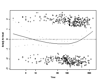
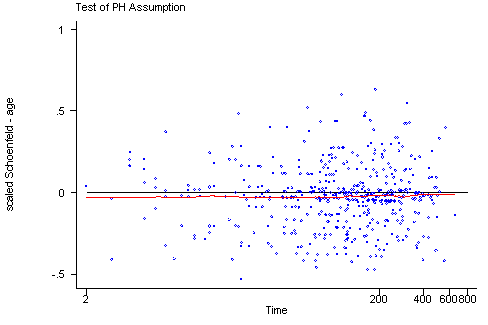
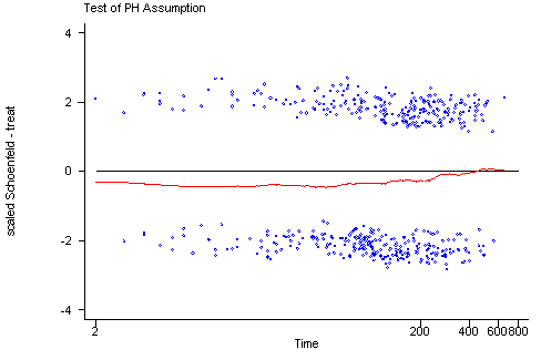
3. Tests and Graps Based on the Schoenfeld Residuals Testing the time dependent covariates is equivalent to testing for a non-zero slope in a generalized linear regression of the scaled Schoenfeld residuals on functions of time. A non-zero slope is an indication of a violation of the proportional hazard assumption. As with any regression it is highly recommended that you look at the graph of the regression in addition to performing the tests of non-zero slopes. There are certain types on non-proportionality that will not be detected by the tests of non-zero slopes alone but that might become obvious when looking at the graphs of the residuals such as nonlinear relationship (i.e. a quadratic fit) between the residuals and the function of time or undue influence of outliers.
SPLUS First we create the coxph object by using the coxph function. To create the plots of the Schoenfeld residuals versus log(time) create a cox.zph object by applying the cox.zph function to the cox.ph object. Then the plot function will automatically create the Schoenfeld residual plots for each of the predictors in the model including a lowess smoothing curve. The order of the residuals in the time.dep.zph object corresponds to the order in which they were entered in the coxph model. To plot one graph at a time use the bracket notation with the number corresponding to the predictor of interest. The abline function adds a reference line at y=0 to the individual plots.
time.dep <- coxph( Surv(time, censor)~age+race+treat+ site+age:site,
            uis, method="breslow", na.action=na.exclude)
time.dep.zph <- cox.zph(table5.11, transform = 'log')
summary(time.dep.zph)
plot(time.dep.zph)

<plots have been omitted>

             rho chisq     p
     age  0.0245 0.283 0.595
    race  0.0601 1.851 0.174
   treat  0.0346 0.597 0.440
    site  0.0355 0.587 0.444
age:site -0.0289 0.385 0.535
  GLOBAL      NA 3.069 0.689
#plots for the predictors: age and treat including the reference line at y=0
plot(time.dep.zph[1])
abline(h=0, lty=3)
plot(time.dep.zph[3])
abline(h=0, lty=3)
STATA The tests of the non-zero slope developed by Therneau and Grambsch for SPLUS have been implemented in STATA in the stphtest command. The algorithms that STATA uses are slightly different from the algorithms used by SPLUS and therefore the results from the two programs might differ slightly. The stphtest with the detail option will perform the tests of each predictor as well as a global test. There are different functions of time available including the identity function, the log of survival time and the rank of the survival times. The stphtest command with the plot option will provide the graphs with a lowess curve. The usual graphing options can be used to include a horizontal reference line at y=0. Unlike the graphs created in SPLUS the graphs in STATA do not include 95% confidence intervals for the lowess curves which makes it more difficult to assess how much the curves may deviate from the y=0 line.
stcox age race treat site agesite, nolog noshow schoenfeld(sch*) scaledsch(sca*)
stphtest, log detail
stphtest, log plot(age) yline(0)
stphtest, log plot(treat) yline(0)

Test of proportional hazards assumption

      Time:  Log(t)
      ----------------------------------------------------------------
                  |       rho            chi2       df       Prob>chi2
      ------------+---------------------------------------------------
      age         |      0.02448         0.28        1         0.5946
      race        |      0.06006         1.85        1         0.1737
      treat       |      0.03464         0.60        1         0.4398
      site        |      0.03551         0.59        1         0.4437
      agesite     |     -0.02890         0.38        1         0.5351
      ------------+---------------------------------------------------
      global test |                      3.07        5         0.6894
      ----------------------------------------------------------------

