Example
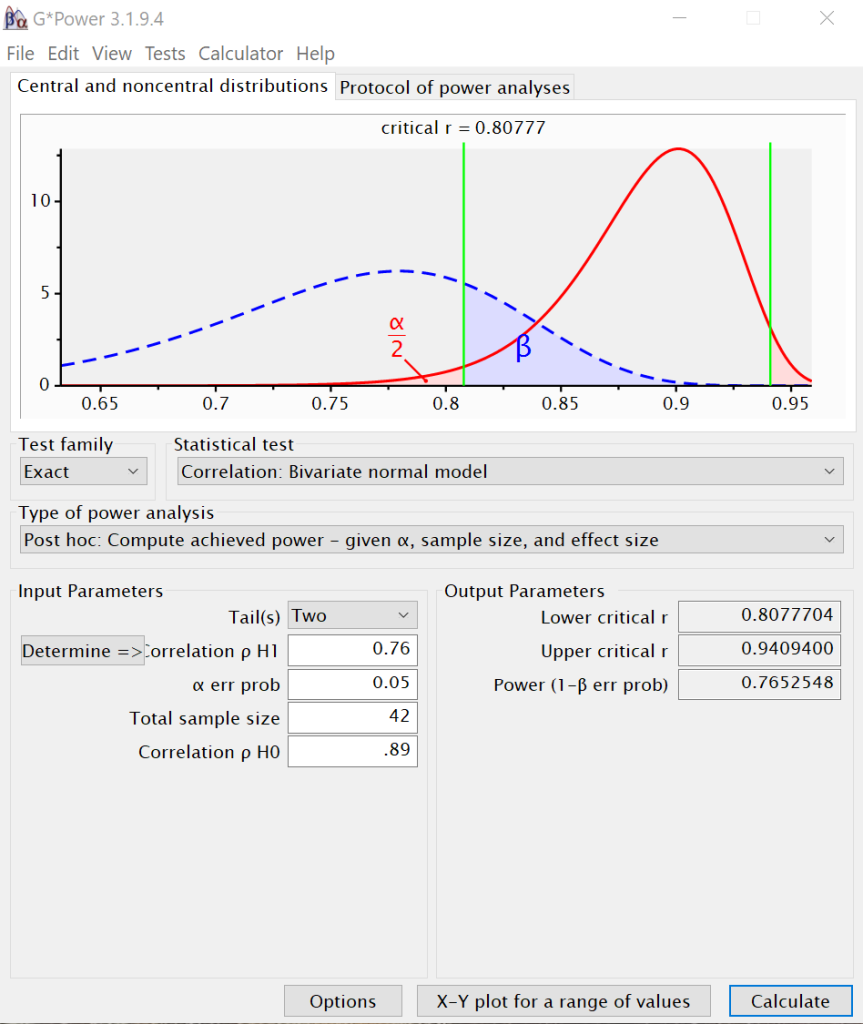
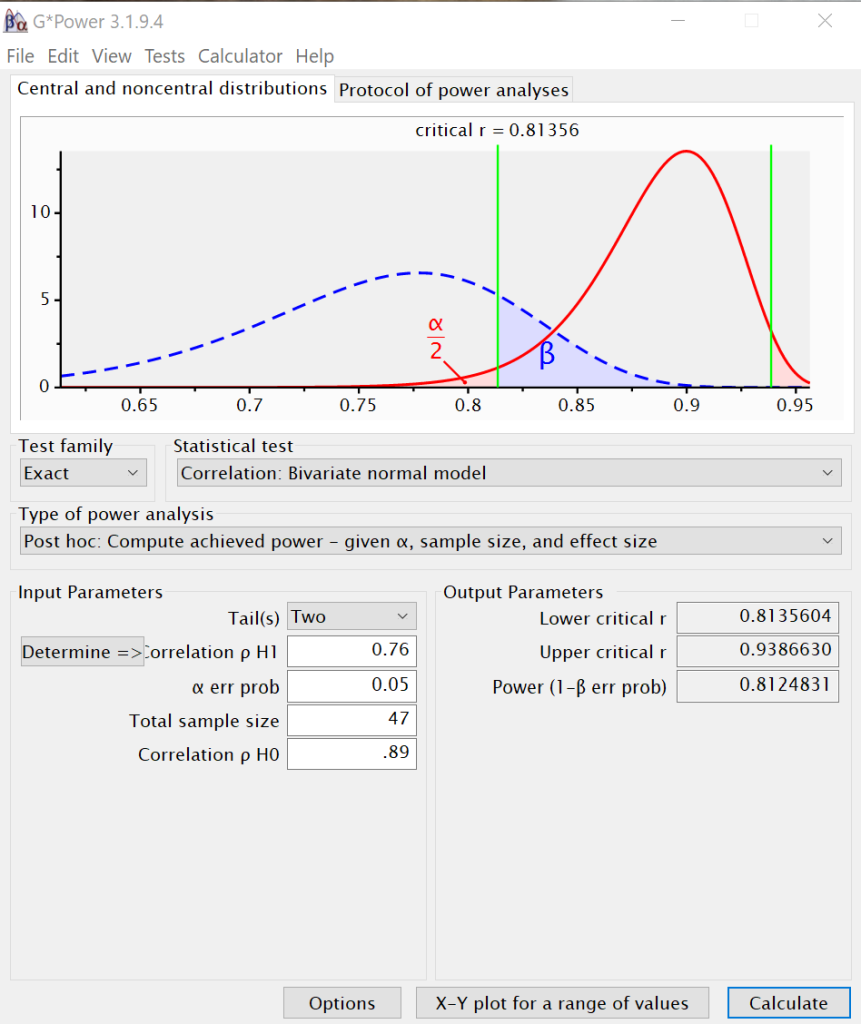
A researcher is trying to develop a new, less expensive, test to detect a particular chemical in soil samples. The old test correlates to the criterion (i.e., gold standard measurement) at r = 0.89. The new test correlates to the criterion at r = 0.76. Two research assistants are asked to collect soil samples to compare the old test with the new test. The first research assistant collects 42 independent soil samples; the second research assistant collects 47 samples. Each runs a power analysis to determine the observed power.
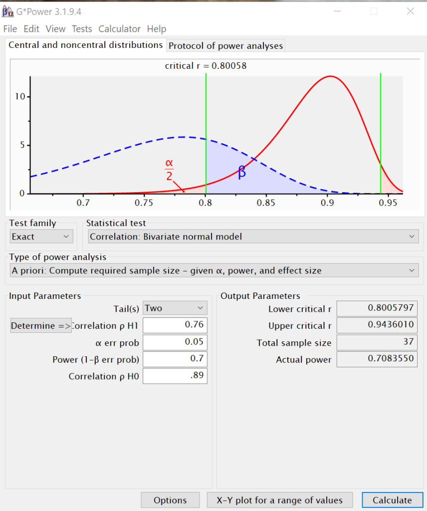
Next, the research assistants are asked to calculate the number of independent samples necessary to detect a difference between 0.89 and 0.76 for power values of .7, .8 and .9.
Prelude to the Power Analysis
There are two different aspects of power analysis. One is to calculate the observed power for a specified sample size as in the first part of the example. The other aspect is to calculate the necessary sample size when given a specific power as in the second part of the example. Technically, power is the probability of rejecting the null hypothesis when the specific alternative hypothesis is true. For all examples, we will assume alpha = 0.05.
Power Analysis
In G*Power, it is fairly straightforward to perform power analysis for comparing correlations. For the first two analyses, we will set the Test Family to Exact and the Statistical Test to Bivariate Normal Model. We will set the type of analysis to “Post hoc” so that we can enter the number of samples each research assistant collected. We set the number of tails to two, the rho for H1 to 0.76, the alpha error probability to 0.05, the total sample size to 42, and the correlation for rho for H0 to 0.86. We then click on Calculate in the lower right-hand corner. We will run the analysis a second time with the value of 47 for the total sample size, the number of samples the second research assistant collected.
We can see that the first research assistant observed a power of approximately 0.76, while the second research assistant observed a power of approximately 0.81. Now the research assistants need to calculate the necessary sample sizes for power values of .7, .8 and .9.
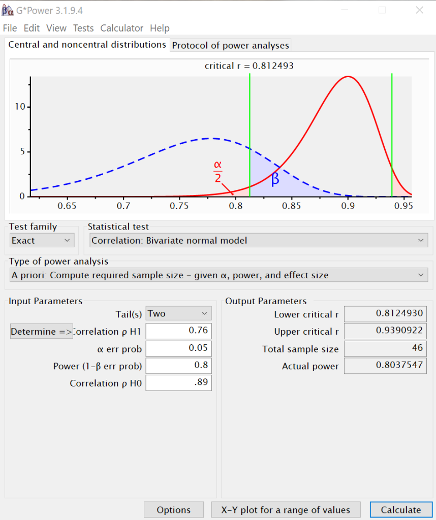
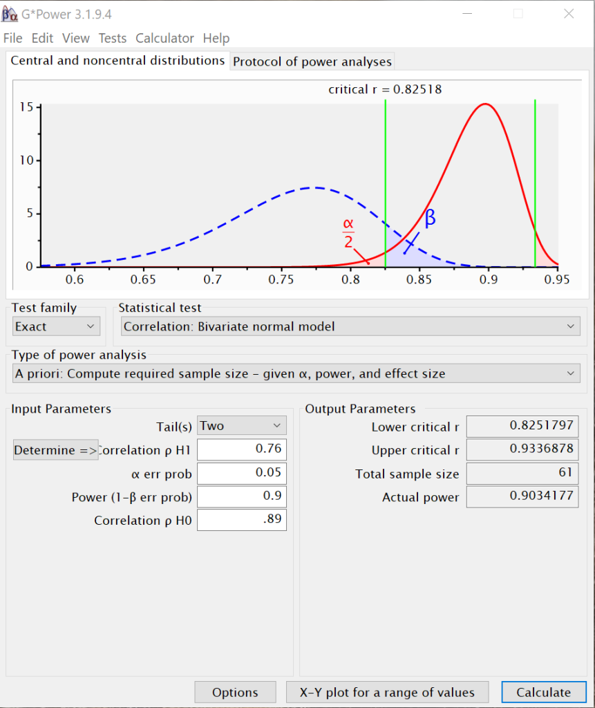 The required sample size for a power of .7 is 37. The required sample size for a power of .8 is 46, and the required sample size for a power of .9 is 61. This makes sense, because as power increases, the sample size must increase, assuming that alpha and the effect size are held constant.

