NOTE: This page was developed using G*Power version 3.0.10. You can download the current version of G*Power from https://www.psychologie.hhu.de/arbeitsgruppen/allgemeine-psychologie-und-arbeitspsychologie/gpower . You can also find help files, the manual and the user guide on this website.
Examples
Example 1. A company that manufactures light bulbs claims that a particular type of light bulb will last 850 hours on average with standard deviation of 50. A consumer protection group thinks that the manufacturer has overestimated the lifespan of their light bulbs by about 40 hours. How many light bulbs does the consumer protection group have to test in order to make their point with reasonable confidence?
Example 2. It has been estimated that the average height of American male adults is 70 inches. I t has also been postulated that there is a positive correlation between height and intelligence. If this is true, then the average height of a male graduate students on campus should be greater than the average height of American male adults in general. To test this theory, one would randomly sample a small group of male graduate students. However, one would need to know how many male graduate students need to measured such that the hypothesis can be reasonable tested.
Prelude to the power analysis
For the power analysis below, we are going to focus on Example 1, testing the average lifespan of a light bulb. Here, the sample size (the number of light bulbs to be tested) is the unknown to be solved for. We will need to identify this variable for a given significance level and power.
A good start would be to list our known values and assumptions. The bulbs’ stated longevity is 850, with detractors claiming 810. In other words, our null hypothesis H0 = 850, and the alternative hypothesis Ha= 810. It is also of great importance to note that the standard deviation is 50, as not all light bulbs are created equal. Additionally, as the test is to show a discrepancy from the null hypothesis and not specifically a greater or lesser value, it is a two-tailed test.
Significance level sets the probability of Type 1 error; the probability that the null hypothesis will be rejected when it is, in fact, true. Conversely, power measures the probability that a Type 2 error will not occur, a Type 2 error being the incidence of a false null hypothesis failing to be rejected. In other words, power is the likelihood of the test appropriately rejecting H0. For this example, we will choose a significance level of .05 and a power of .9.
Power analysis
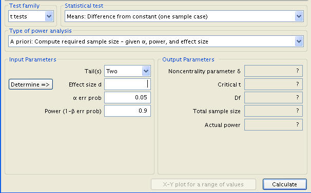
Immediately, we can put our known measures into G*Power’s interface.

We begin by indicating that we are performing a t-test, and, more specifically, a means test involving a sample’s difference from a constant (how much do the reality of the bulbs differ from the manufacturer’s claim of 850 hours?).
The type of power analysis being performed is noted to be an ‘A Priori’ analysis, a determination of sample size. From there, we can input the number of tails, the value of our chosen significance level (α), and the power; 2, .05, and .9, respectively. The only input still requested is the effect size, or the difference of the null and hypothetical means divided by the standard deviation.
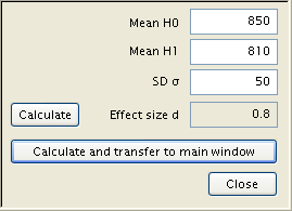
By clicking on the ‘Determine’ button to the left of the Effect size input, a new set of input cells is called up, for the null hypothesis mean (here represented as Mean H0), the alternative mean (Mean H1), and the standard deviation (SD σ). As these numbers are known to us (850, 810, and 50), simply type them in and click ‘Calculate and transfer to main window’. As a result, the effect level’s value (given as .8) is handily computed and inputted.
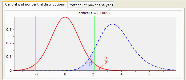
From there, a press of the ‘Calculate’ button in the main window produces the desired sample size, among other statistics. These are, in descending order, the Noncentrality parameter δ, the Critical t (the number of standard deviations from the null mean where an observation becomes statistically significant), the number of degrees freedom, and the test’s actual power. In addition, a graphical representation of the test is shown, with the sampling distribution a dotted blue line, the population distribution represented by a solid red line, a red shaded area delineating the probability of a type 1 error, a blue area the type 2 error, and a pair of green lines evocating the critical points t.
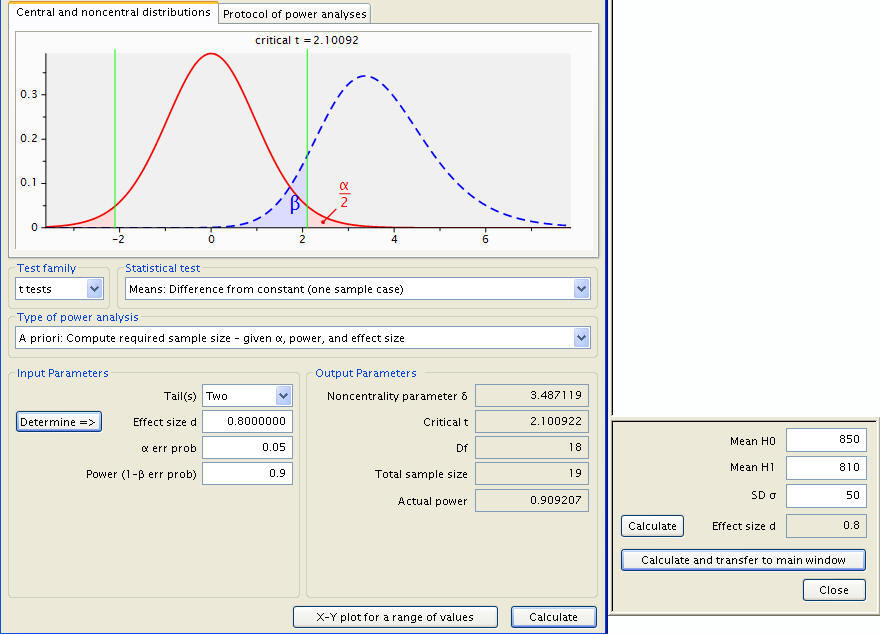
To at last answer our question, the sample size is shown to be 19. Thus, no fewer than nineteen light bulbs must be tested in order to generate a statistically significant result (suggesting a rejection of the null hypothesis, the manufacturer’s claim) with a power of .9.
To twist the initial question around, supposing only 10 light bulbs were available for testing, what power would the test have, all else held constant?
This can be determined simply. The frame of the question is altered by setting the type of power analysis from the ‘A Priori’ search for sample size to a ‘Post hoc’ pursuit of achieved power. Immediately, the input parameters readjust to replace the power input with one for sample size. As all other variables remain as previous, the new measure of sample size, 10, is entered in.
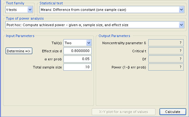
Making use of the Calculate button, we receive the new output parameters.
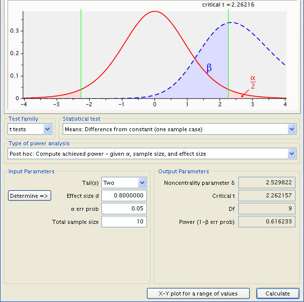
These include the Noncentrality parameter δ, the Critical t, and the degrees freedom as before, in addition to Power, here measuring 0.616233, having decreased from .9 due to the smaller sample.
Discussion
In reference to the initial question and its outcome, it is important to note that the test takes effect size into account, rather than the means themselves. As such, a null mean of 850 and an alternative mean of 810 are considered identical to a null mean of 810 and an alternative mean of 850, and are represented the same graphically. Thus, the graph displayed for our example is in fact a mirror image of what it should actually be, the null distribution being incorrectly to the left of the sampling distribution. It remains important to consider the numbers themselves and not be unduly misled.
As seen in the second half of the analysis, by adjusting the type of power analysis according to the values given and the values unknown, the requested output can be generated for an unknown effect size, significance level, and implied significance level with power, as well as the demonstrated ability to perform power and sample size calculations. In all cases, the unknown variable should properly designated, followed by entering the givens in the input parameters.

For more information on power analysis, please visit our Introduction to Power Analysis seminar.
