NOTE: This page was developed using G*Power version 3.0.10. You can download the current version of G*Power from http://www.psycho.uni-duesseldorf.de/abteilungen/aap/gpower3/ . You can also find help files, the manual and the user guide on this website.
Examples
Example 1. A company markets an eight week long weight loss program and claims that at the end of the program, on average, a participant will have lost 5 pounds. On the other hand, you have studied the program and you believe that their program is scientifically unsound and shouldn’t work at all. With some limited funding at hand, you want test the hypothesis that the weight loss program does not help people lose weight. Your plan is to get a random sample of people and put them on the program. You will measure their weight at the beginning of the program and then measure their weight again at the end of the program. Based on some previous research, you believe that the standard deviation of the weight difference over eight weeks will be 5 pounds. You now want to know how many people you should enroll in the program to test your hypothesis.
Example 2. A human factors researcher wants to study the difference between dominant hand and the non-dominant hand in terms of manual dexterity. She designs an experiment where each subject would place 10 small beads on the table in a bowl, once with the dominant hand and once with the non-dominant hand. She measured the number seconds needed in each round to complete the task. She has also decided that the order in which the two hands are measured should be counter balanced. She expects that the average difference in time would be 5 seconds with the dominant hand being more efficient with standard deviation of 10. She collects her data on a sample of 35 subjects. The question is, what is the statistical power of her design with an N of 35 to detect the difference in the magnitude of 5 seconds.
Prelude to the power analysis
In both of the examples, there are two measures on each subject, and we are interested in the mean of the difference of the two measures. This can be done with a t-test for paired samples (dependent samples). In a power analysis, there are always a pair of hypotheses: a specific null hypothesis and a specific alternative hypothesis. For instance, in Example 1, the null hypothesis is that the mean weight loss is 5 pounds and the alternative is zero pounds. In Example 2, the null hypothesis is that mean difference is zero seconds and the alternative hypothesis is that the mean difference is 5 seconds.
There are two different aspects of power analysis. One is to calculate the necessary sample size for a specified power. The other aspect is to calculate the power when given a specific sample size. Technically, power is the probability of rejecting the null hypothesis when the specific alternative hypothesis is true.
Both of these calculations depend on the Type I error rate, the significance level. The significance level (called alpha), or the Type I error rate, is the probability of rejecting H0 when it is actually true. The smaller the Type I error rate, the larger the sample size required for the same power. Likewise, the smaller the Type I error rate, the smaller the power for the same sample size. This is the trade-off between the reliability and sensitivity of the test.
Power analysis
Immediately, we set G*Power to test the difference between two sample means.

The type of power analysis being performed is noted to be an ‘A Priori’ analysis, a determination of sample size. From there, we can input the number of tails, the value of our chosen significance level (α), and whatever power desired. For the purposes of Example 1, let us choose the default significance level of .05 and a power of .8.
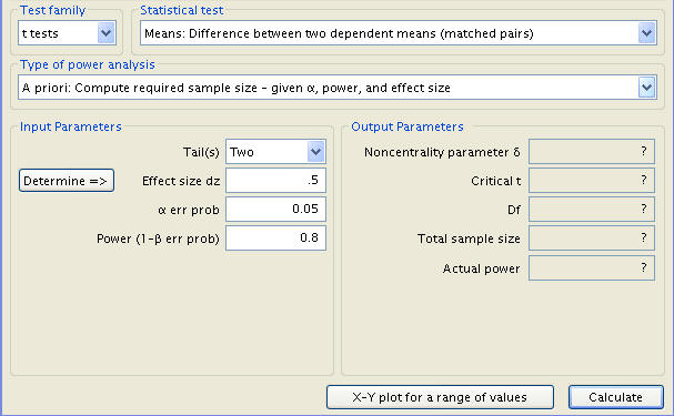
All that remains to be inputted is the effect size, which can be determined by using the appropriately named ‘Determine’ button. This calls up a side window in which we can indicate that we wish to gauge effect size from differences (rather than group parameters), and then entering the mean of difference (which is to say the difference between the null and alternative hypotheses means, 5 pounds), as well as the standard deviation (5 pounds).
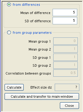
A click of ‘Calculate and transfer to main window’ solves for the effect size, here 1. As the inputs are now all assembled, the ‘Calculate’ button produces the desired necessary sample size, among other statistics. These are, in descending order, the Noncentrality parameter δ, the Critical t (the number of standard deviations from the null mean where an observation becomes statistically significant), the number of degrees freedom, and the test’s actual power. In addition, a graphical representation of the test is shown, with the sampling distribution a dotted blue line, the population distribution represented by a solid red line, a red shaded area delineating the probability of a type 1 error, a blue area the type 2 error, and a pair of green lines demarcating the critical points t.
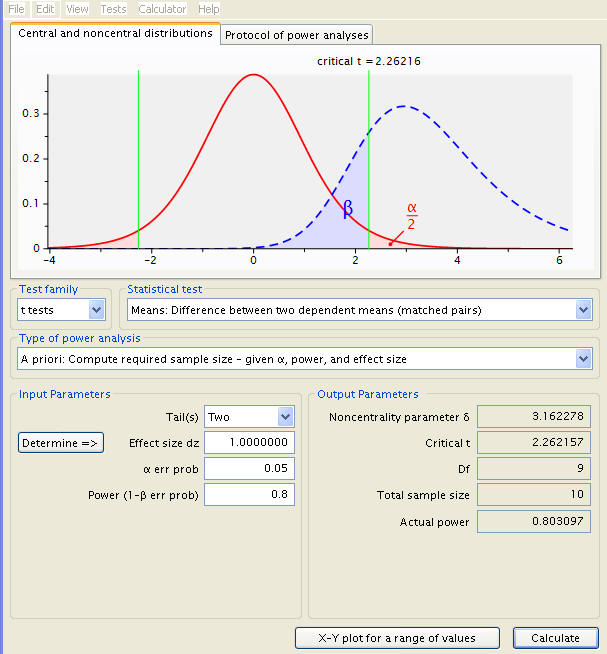
Thus, we arrive at a sample size of 10, meaning ten people would need to be enrolled in the weight loss program to test the hypothesis at significance level .05 and power .8. What would happen at a higher power level, all else held constant?
This is a simple enough measure to adjust, simply enter a different number into the power input and calculate anew. To demonstrate (with .85 and .09):
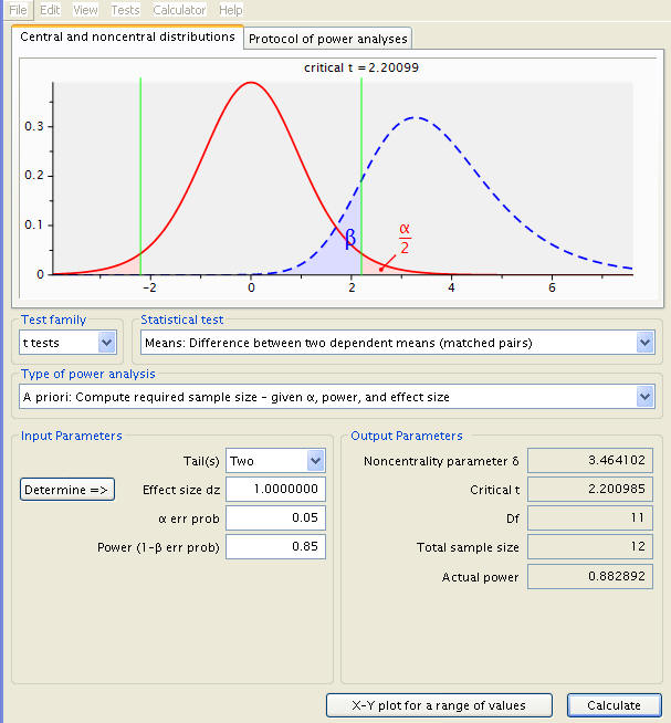
At a power of .85, the necessary sample size increases to twelve.
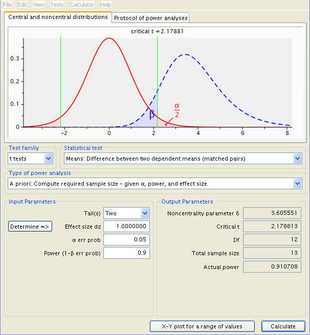
At a power of .9, the necessary sample size increases further, to thirteen. An increase in power clearly requires an increase in sample size.
Now, given a power of .9107 (the actual power for the last calculation), what happens to sample size with the significance level changed to .01? The answer can be swiftly deduced with a new set of inputs.
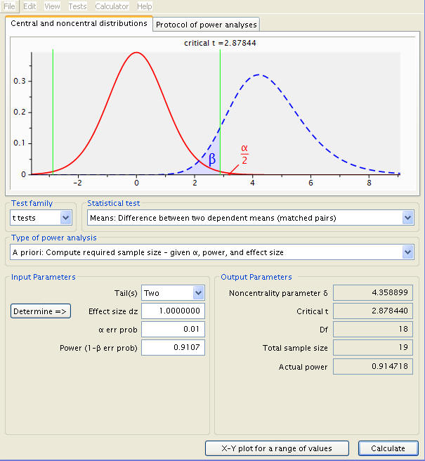
Sample size has swelled to 19. It would seem that to reduce the likelihood of type 1 error, a larger sample size is called for. Additionally, it is important to consider that all our calculations so far have been done under the assumption that the data are normally distributed. If this is not the case, a still larger sample is needed.
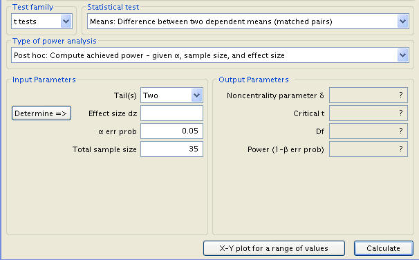
Turning to Example 2, we find our priorities rearranged. Sample size is given as 35 people, but power is unknown. To manage this, the type of power analysis is changed from the ‘A Priori’ investigation of sample size to the ‘Post Hoc’ power calculation. A couple new variables are to be inputted; the sample size is new and the significance level has been restored to .05.
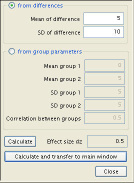
Effect size must be redefined, with the difference given as 5 seconds and a standard deviation of 10.
The necessary inputs now in place, we can calculate the test’s power.
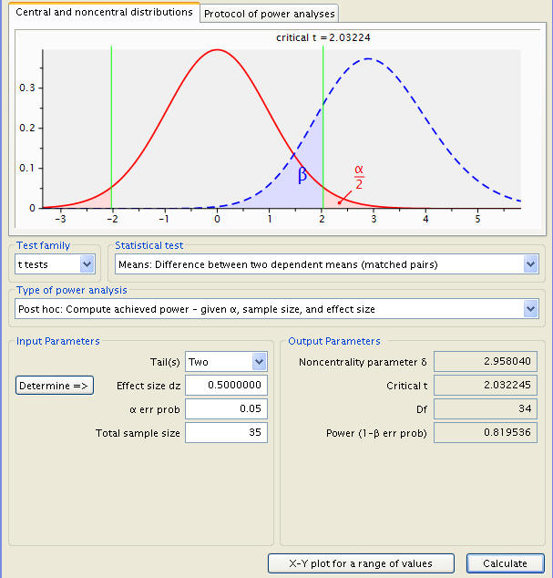
The power is found to be .819536. In other words, a five-second difference in timing will be picked up on roughly 82% of the time.
Note, however, that the previous test had two tails, meaning a simple difference in means is looked for, and not one being specifically greater than the other. However, as the experiment concerns the relative strength of a dominant hand to its counterpart, it can be assumed that the former is always better than the latter, and a one-tailed test can be conducted. A simple shift of the ‘Tail(s)’ input parameter and a click of the ‘Calculate’ button produces this:
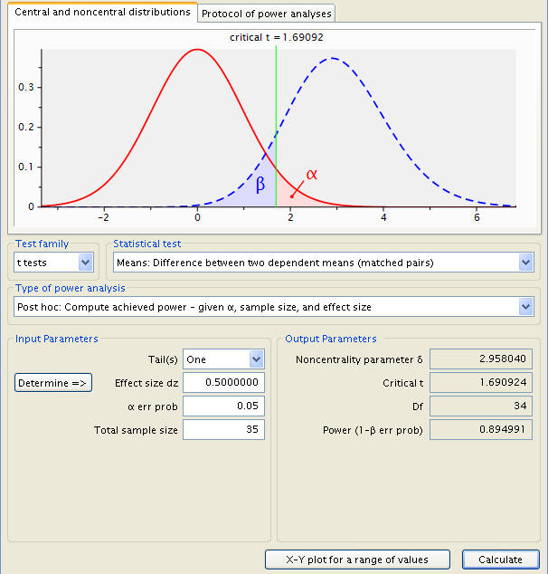
Here, power is found to be .894991.
Note also that G*Power is capable of performing power and sample size given more specific initial conditions. Supposing that for Example 2, the correlation between left and right hand measures is in fact .9 instead of the .5 implicitly assumed in calculating effect size from differences. We are looking for sample size (an ‘A Priori’ power analysis), and setting power, significance level, and the number of tails are to familiar levels (.8, .05, and 2, respectively), but changing the method of effect size determination to ‘from group parameters’.
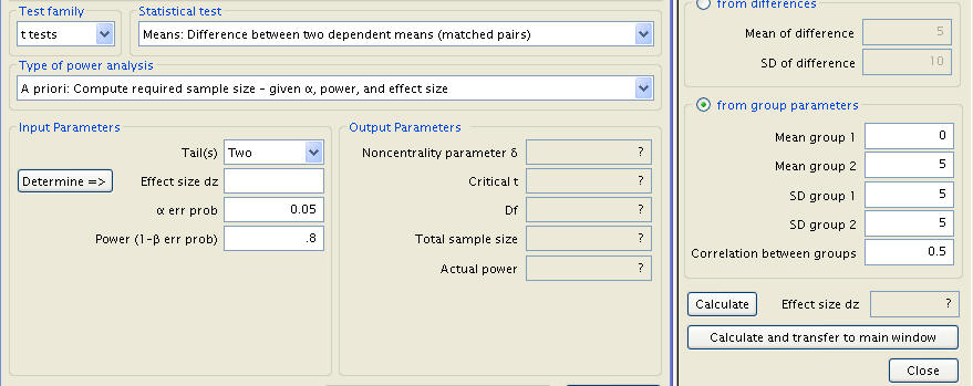
The two standard deviations are assumed identical at 10, the means of groups 1 and 2 can be anything so long as the difference between them is 5 (any values obeying this rule will be shown as graphically identical, a point which should be noted as potentially misleading). The variable of importance, correlation between groups, is set to the predetermined value of .9. The sum total of this new sequence of inputs is an effect size of 1.118034.
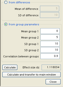
A press of ‘Calculate and transfer to main window’, followed by the main window’s ‘Calculate’, produces the new sample size.
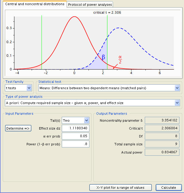
What required ten people in the initial example has been scaled down to nine with a stronger correlation between the two measurements. The closer the two measures are, the smaller the necessary sample.
The group parameters input is also useful for measurements with varying standard deviations between two groups, as evidenced in the following retread of Example 1. Assuming that the standard deviation for the pre-program group is 7, with the post-program standard deviation at 12 and a correlation of .5, the resultant sample size can be calculated. The vital edits are made within the window called by the ‘Determine’ button, within the group parameters input.
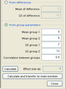
Moving to the main window and calculating, the numbers needed for this setting can be deduced.

With an initial standard deviation of 7, a follow-up deviation of 12, and a correlation of .5, 37 people will be needed.
Discussion
One major technical assumption is the normality assumption. If the distribution is skewed, then a small sample size may not have the power shown in the results, because the value in the results is calculated using the method based on the normality assumption. It might not even be a good idea to do a t-test on a small sample to begin with.
What we really need to know is the difference between the two means, not the individual values. In fact, what really matters, is the difference of the means over the pooled standard deviation. We call this the effect size. It is usually not an easy task to determine the effect size. It usually comes from studying the existing literature or from pilot studies. A good estimate of the effect size is the key to a successful power analysis.
For more information on power analysis, please visit our Introduction to Power Analysis seminar.
