NOTE: This page was developed using G*Power version 3.0.10. You can download the current version of G*Power from http://www.psycho.uni-duesseldorf.de/abteilungen/aap/gpower3/ . You can also find help files, the manual and the user guide on this website.
Examples
Example 1. A clinical dietician wants to compare two different diets, A and B, for diabetic patients. She hypothesizes that diet A (Group 1) will be better than diet B (Group 2), in terms of lower blood glucose. She plans to get a random sample of diabetic patients and randomly assign them to one of the two diets. At the end of the experiment, which lasts 6 weeks, a fasting blood glucose test will be conducted on each patient. She also expects that the average difference in blood glucose measure between the two group will be about 10 mg/dl. Furthermore, she also assumes the standard deviation of blood glucose distribution for diet A to be 15 and the standard deviation for diet B to be 17. The dietician wants to know the number of subjects needed in each group assuming equal sized groups.
Example 2. An audiologist wanted to study the effect of gender on the response time to a certain sound frequency. He suspected that men were better at detecting this type of sound then were women. He took a random sample of 20 male and 20 female subjects for this experiment. Each subject was be given a button to press when he/she heard the sound. The audiologist then measured the response time – the time between the sound was emitted and the time the button was pressed. Now, he wants to know what the statistical power is based on his total of 40 subjects to detect the gender difference.
Prelude to the power analysis
There are two different aspects of power analysis. One is to calculate the necessary sample size for a specified power as in Example 1. The other aspect is to calculate the power when given a specific sample size as in Example 2. Technically, power is the probability of rejecting the null hypothesis when the specific alternative hypothesis is true.
For the power analyses below, we are going to focus on Example 1, calculating the sample size for a given statistical power of testing the difference in the effect of diet A and diet B. Notice the assumptions that the dietician has made in order to perform the power analysis. Here is the information we have to know or have to assume in order to perform the power analysis:
- The expected difference in the average blood glucose; in this case it is set to 10.
- The standard deviations of blood glucose for Group 1 and Group 2; in this case, they are set to 15 and 17 respectively.
- The alpha level, or the Type I error rate, which is the probability of rejecting the null hypothesis when it is actually true. A common practice is to set it at the .05 level.
- The pre-specified level of statistical power for calculating the sample size; this will be set to .8.
- The pre-specified number of subjects for calculating the statistical power; this is the situation for Example 2.
Notice that in the first example, the dietician didn’t specify the mean for each group, instead she only specified the difference of the two means. This is because that she is only interested in the difference, and it does not matter what the means are as long as the difference is the same.
Power analysis
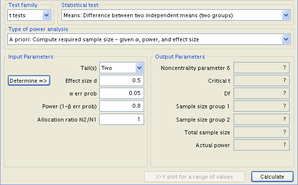
In G*Power, it is fairly straightforward to perform power analysis for comparing means. Approaching Example 1, first we set G*Power to a t-test involving the difference between two independent means.

As we are searching for sample size, an ‘A Priori’ power analysis is appropriate. As significance level and power are given, we are free to input those values, which are .05 and .8, respectively. Additionally, equal sized sample groups are assumed, meaning the allocation ratio of N1 to N2 is 1.
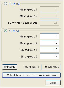
All that remains to be accounted for is the effect size. A click of the ‘Determine’ button calls up the appropriate window. The specific numbers entered for the means of groups 1 and 2 are irrelevant, so long as the difference between them is the correct value, in our case 10. Thus, 0 and 10, 5 and 15, -2 and 8, etc., would all be acceptable. For simplicity we will set the mean of group 1 to 0 and the mean of group 2 to 10. The respective standard deviations are known to us, as 15 and 17. Once entered, a press of ‘Calculate and transfer to main window’ inputs the effect size.
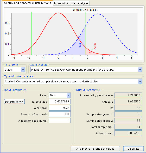
From there, a click of ‘Calculate’ in the main window produces the desired result, along with, in descending order, the Noncentrality parameter δ, the Critical t (the number of standard deviations from the null mean where an observation becomes statistically significant), the number of degrees freedom, and the test’s actual power. In addition, a graphical representation of the test is shown, with the sampling distribution a dotted blue line, the population distribution represented by a solid red line, a red shaded area delineating the probability of a type 1 error, a blue area the type 2 error, and a pair of green lines demarcating the critical points t.
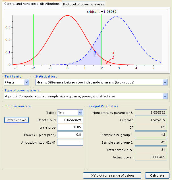
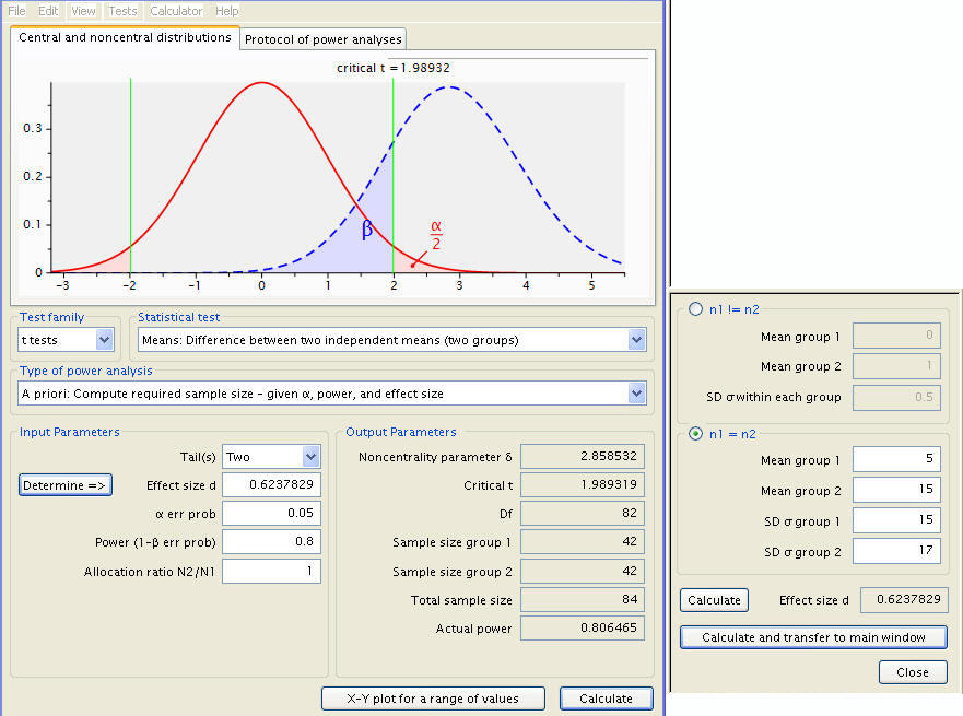
The calculation results indicate that we need 42 subjects for diet A and another 42 subject for diet B in our sample in order to measure the effect. Now, let’s use another pair of means with the same difference. As we have discussed earlier, the results should be the same, and indeed they are.
Now the dietician may feel that a total sample size of 84 subjects is beyond her budget. One way of reducing the sample size is to increase the Type I error rate, or the alpha level. Let’s say instead of using alpha level of .05 we will use .07. Then our sample size will reduce by 4 for each group as shown below.
Now suppose the dietician can only collect data on 60 subjects with 30 in each group. What will the statistical power for her t-test be with respect to alpha level of .05?
To manage this, the type of power analysis is changed from the ‘A Priori’ investigation of sample size to the ‘Post Hoc’ power calculation. A couple new variables are to be inputted; the sample sizes are new and the significance level has been restored to .05.
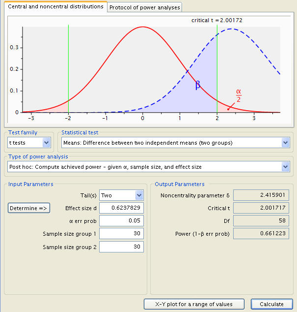
The power is .661223.
What if she actually collected her data on 60 subjects but with 40 on diet A and 20 on diet B instead of equal sample sizes in the groups?
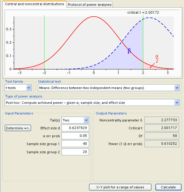
As you can see the power goes down from .661223 to .610252 even though the total number of subjects is the same; a balanced design is more efficient.
Discussion
An important technical assumption is the normality assumption. If the distribution is skewed, then a small sample size may not have the power shown in the results, because the value in the results is calculated using the method based on the normality assumption. We have seen that in order to compute the power or the sample size, we have to make a number of assumptions. These assumptions are used not only for the purpose of calculation, but are also used in the actual t-test itself. So one important side benefit of performing power analysis is to help us to better understand our designs and our hypotheses.
We have seen in the power calculation process that what matters in the two-independent sample t-test is the difference in the means and the standard deviations for the two groups. This leads to the concept of effect size. In this case, the effect size will be the difference in means over the pooled standard deviation. The larger the effect size, the larger the power for a given sample size. Or, the larger the effect size, the smaller sample size needed to achieve the same power. So, a good estimate of effect size is the key to a good power analysis. However, it is not always an easy task to determine the effect size. Good estimates of effect size come from the existing literature or from pilot studies.
For more information on power analysis, please visit our Introduction to Power Analysis seminar.
