NOTE: This page was developed using G*Power version 3.0.10. You can download the current version of G*Power from http://www.psycho.uni-duesseldorf.de/abteilungen/aap/gpower3/ . You can also find help files, the manual and the user guide on this website.
Introduction
Power analysis is the name given to the process of determining the sample size for a research study. The technical definition of power is that it is the probability of detecting an effect when it exists. Many students think that there is a simple formula for determining sample size for every research situation. However, the reality is that there are many research situations that are so complex that they almost defy rational power analysis. In most cases, power analysis involves a number of simplifying assumptions, in order to make the problem tractable, and running the analyses numerous times with different variations to cover all of the contingencies.
In this page we will try to illustrate how to do a power analysis for a test of two independent proportions, i.e., the response variable has two levels and the predictor variable also has two levels. Instead of analyzing these data using a test of independent proportions, we could compute a chi-square statistic in a 2×2 contingency table or run a simple logistic regression analysis. These three analyses yield the same results and would require the same sample sizes to test effects.
Description of the experiment
It is known that a certain type of skin lesion will develop into cancer in 30% of patients if left untreated. There is a drug on the market that will reduce the probability of cancer developing to 20%. . A pharmaceutical company is developing a new drug to treat skin lesions, but it will only be worthwhile to do so if the new drug reduces the probability of developing cancer to 15% or better. The pharmaceutical company plans to do a study with patients randomly assigned to two groups, the control (untreated) group and the treatment group. The company wants to know how many subjects will be needed to test a difference in proportions of .15 with a power of .8 at alpha equal to .05.
The power analysis
G*Power is easily capable of determining the sample size needed for tests of two independent proportions as well as for tests of means. To begin, the program should be set to the z family of tests, to a test of proportions, and to perform the ‘A Priori’ power analysis necessary to identify sample size.

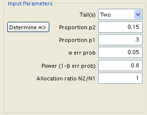
From there, simply input the necessary parameters. We are given the power, significance level, and the values of the two proportions, and we can assume that we want equally sized sample groups (an allocation ratio of 1).
Pressing ‘Calculate’ produces the desired results along with the critical z (the number of standard deviations from the null mean where an observation becomes statistically significant) and the test’s actual power. In addition, a graphical representation of the test is shown, with distribution of the test statistics, given difference between proportions (i.e. p2 – p1 = 0.15 – 0.3 = -0.15) as a dotted blue line and distribution of the test statistics, given difference between proportions equal to zero represented by a solid red line. A red shaded area delineating the probability of a type 1 error, a blue area the type 2 error, and a pair of green lines demarcating the critical points z.
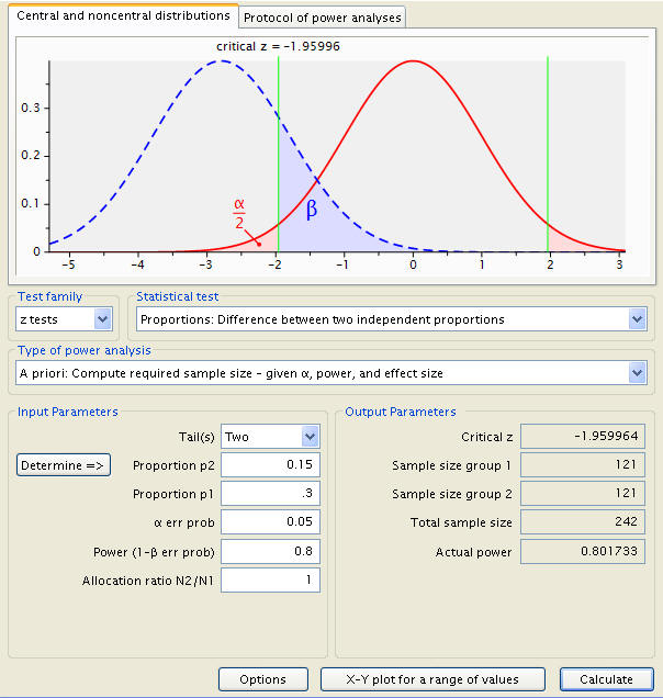
Each group will require 121 people.
This is all well and good, but a two-sided test doesn’t make much sense in this situation. We want to test for a drug that reduces the probability of cancer not for one that increases the probability. In this case we might want to use a one-tail test, adjustable easily enough by changing the input in ‘Tail(s)’.
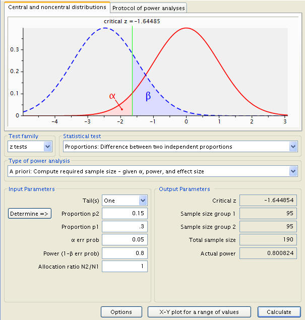
G*Power indicates that we need to use 95 subjects in each group to find a change in probability of .15 for a power of .8 when alpha equals .05.
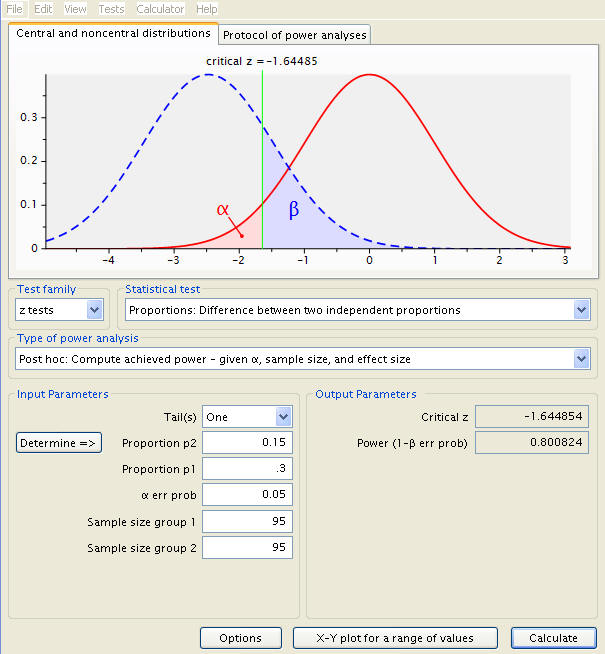
Just as a check, let’s run the analysis specifying each of the two sample sizes. This is accomplished by changing the type of power analysis from the ‘A Priori’ investigation of sample size to the ‘Post Hoc’ power calculation. The solved-for sample sizes should be automatically tabulated.
Now, because we believe that we know a lot about the incidence of cancer in the untreated group, we would like to make the control group half as large as the treatment group. We can easily do this by adjusting the allocation ratio input. As we desire the control group (group 1) to be half as large as the treatment group (group 2), N2/N1 should equal 2.
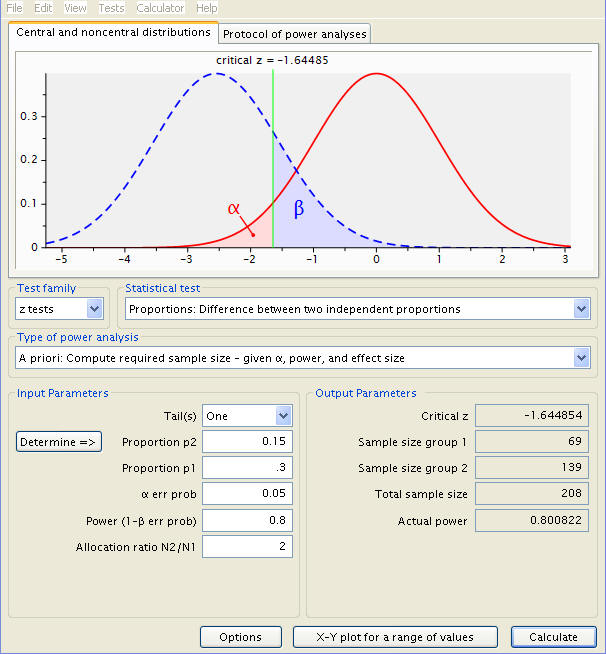
With this unbalanced design we have an estimated power of 0.800822, which the company deems acceptable.
For more information on power analysis, please visit our Introduction to Power Analysis seminar.
