Table 2.3 on page 27.
We are going to use two SPSS files. The level-1 file imm10.sav and the level-2 file imm10_lev2.sav. We also assume that one has already created an SSM file based on these two files. For help on how to create an SSM file based on these SPSS files, we refer to HLM manual.
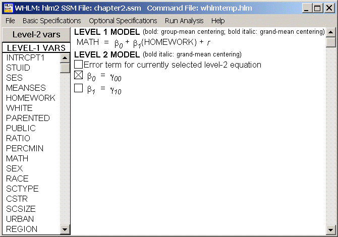
This is just a level-1 OLS regression. Variable HOMEWORK is used as uncentered and it is fixed as well as the intercept.

The output is as follows. Some of the output is omitted.
The outcome variable is MATH
  The model specified for the fixed effects was:
 ----------------------------------------------------
   Level-1                  Level-2
   Coefficients             Predictors
 ----------------------   ---------------
#        INTRCPT1, B0      INTRCPT2, G00
#  HOMEWORK slope, B1      INTRCPT2, G10
'#' - The residual parameter variance for this level-1 coefficient has been set
      to zero.
 The model specified for the covariance components was:
 ---------------------------------------------------------
Sigma squared (constant across level-2 units)
 Summary of the model specified (in equation format)
 ---------------------------------------------------
Level-1 Model
Y = B0 + B1*(HOMEWORK) + R
Level-2 Model
	B0 = G00
	B1 = G10
 Least Squares Estimates
 -----------------------
sigma_squared = 93.73176
The outcome variable is MATH
 Least-squares estimates of fixed effects
 ----------------------------------------------------------------------------
                                       Standard
    Fixed Effect         Coefficient   Error      T-ratio   d.f.     P-value
 ----------------------------------------------------------------------------
 For       INTRCPT1, B0
    INTRCPT2, G00          44.073860   0.988641    44.580       258    0.000
 For HOMEWORK slope, B1
    INTRCPT2, G10           3.571856   0.388237     9.200       258    0.000
 ----------------------------------------------------------------------------
The outcome variable is MATH
 Least-squares estimates of fixed effects
 (with robust standard errors)
 ----------------------------------------------------------------------------
                                       Standard
    Fixed Effect         Coefficient   Error      T-ratio   d.f.     P-value
 ----------------------------------------------------------------------------
 For       INTRCPT1, B0
    INTRCPT2, G00          44.073860   2.113577    20.853       258    0.000
 For HOMEWORK slope, B1
    INTRCPT2, G10           3.571856   0.728682     4.902       258    0.000
 ----------------------------------------------------------------------------
The robust standard errors are appropriate for datasets having a moderate to
large number of level 2 units.  These data do not meet this criterion.
 The least-squares likelihood value = -957.799219
 Deviance =   1915.59844
 Number of estimated parameters =    1
 The outcome variable is     MATH
 Least-squares estimates of fixed effects
 (with robust standard errors)
 ----------------------------------------------------------------------------
                                       Standard
    Fixed Effect         Coefficient   Error      T-ratio   d.f.     P-value
 ----------------------------------------------------------------------------
 For       INTRCPT1, B0
    INTRCPT2, G00          44.073860   2.113577    20.853       258    0.000
 For HOMEWORK slope, B1
    INTRCPT2, G10           3.571856   0.728682     4.902       258    0.000
 ----------------------------------------------------------------------------
Table 2.4 on page 28.
This is a level-1 weighted OLS regression. In order to do so in HLM, we have to create a level-1 data file with aggregated data on the ten selected schools. We created this data file in SPSS and called it table2_4.sav and it looks like:
schid     mmath       mhwk     weight
 7472    45.7391    1.39130      23
 7829    42.1500    2.35000      20
 7930    53.2500    1.83333      24
24725    43.5455    1.63636      22
25456    49.8636    0.86364      22
25642    46.4000    1.15000      20
62821    62.8209    3.29851      67
68448    49.6667    2.09524      21
68493    46.3333    1.33333      21
72292    47.8500    1.60000      20
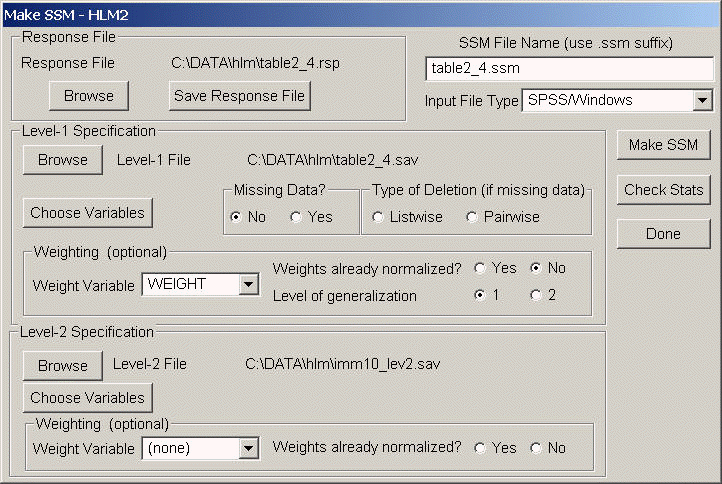
We need to create a new SSM file based on table2_4.sav and imm10_lev2.sav and variable weight is used as weight variable at level 1 un-normalized. One would have to say, this is a lot of work to do a level-1 regression. We could have done it easily in SPSS for that matter. The point we want to make here is that HLM has the ability to take care a weight variable.

The model specification and the output is shown below. Some of the output has been omitted.
Summary of the model specified (in equation format)
 ---------------------------------------------------
Level-1 Model
Y = B0 + B1*(MHWK) + R
Level-2 Model
	B0 = G00
	B1 = G10
 Least Squares Estimates
 -----------------------
sigma_squared = 24.17109
The outcome variable is MMATH
 Least-squares estimates of fixed effects
 ----------------------------------------------------------------------------
                                       Standard
    Fixed Effect         Coefficient   Error      T-ratio   d.f.     P-value
 ----------------------------------------------------------------------------
 For       INTRCPT1, B0
    INTRCPT2, G00          37.108633   4.058993     9.142         8    0.000
 For     MHWK slope, B1
    INTRCPT2, G10           7.014745   1.853336     3.785         8    0.006
 ----------------------------------------------------------------------------
The outcome variable is MMATH
 Least-squares estimates of fixed effects
 (with robust standard errors)
 ----------------------------------------------------------------------------
                                       Standard
    Fixed Effect         Coefficient   Error      T-ratio   d.f.     P-value
 ----------------------------------------------------------------------------
 For       INTRCPT1, B0
    INTRCPT2, G00          37.108633   3.225961    11.503         8    0.000
 For     MHWK slope, B1
    INTRCPT2, G10           7.014745   1.602668     4.377         8    0.002
 ----------------------------------------------------------------------------
Table 2.5 on page 29.
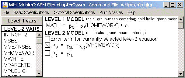
We go back to our original two files, imm10.sav and imm10_lev2.sav and use the same SSM file created for Table 2.3. We can simply use out old chapter2.ssm file and the only thing we have to do is to select our model. The model specified is shown in its equation format and the parameter estimates are shown below.

 Summary of the model specified (in equation format)
 ---------------------------------------------------
Level-1 Model
Y = B0 + B1*(HOMEWORK) + R
Level-2 Model
	B0 = G00 + G01*(MHOMEWOR)
	B1 = G10
 Least Squares Estimates
 -----------------------
sigma_squared = 82.14002
The outcome variable is MATH
 Least-squares estimates of fixed effects
 ----------------------------------------------------------------------------
                                       Standard
    Fixed Effect         Coefficient   Error      T-ratio   d.f.     P-value
 ----------------------------------------------------------------------------
 For       INTRCPT1, B0
    INTRCPT2, G00          37.108633   1.467442    25.288       257    0.000
    MHOMEWOR, G01           4.878110   0.797556     6.116       257    0.000
 For HOMEWORK slope, B1
    INTRCPT2, G10           2.136635   0.432608     4.939       257    0.000
 ----------------------------------------------------------------------------
Table 2.6 on page 30 using the same SSM file.
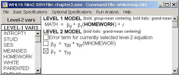
The only difference between this model and the previous one is that variable HOMEWORK is now re-entered into the model as group-mean centered. The estimates are shown below.

  The model specified for the fixed effects was:
 ----------------------------------------------------
   Level-1                  Level-2
   Coefficients             Predictors
 ----------------------   ---------------
#        INTRCPT1, B0      INTRCPT2, G00
                           MHOMEWOR, G01
 * HOMEWORK slope, B1      INTRCPT2, G10
'#' - The residual parameter variance for this level-1 coefficient has been set
      to zero.
'*' - This level-1 predictor has been centered around its group mean.
 Summary of the model specified (in equation format)
 ---------------------------------------------------
Level-1 Model
Y = B0 + B1*(HOMEWORK) + R
Level-2 Model
	B0 = G00 + G01*(MHOMEWOR)
	B1 = G10 + U1
The average OLS level-1 coefficient for HOMEWORK = 1.96094
 Least Squares Estimates
 -----------------------
sigma_squared = 82.14002
The outcome variable is MATH
 Least-squares estimates of fixed effects
 ----------------------------------------------------------------------------
                                       Standard
    Fixed Effect         Coefficient   Error      T-ratio   d.f.     P-value
 ----------------------------------------------------------------------------
 For       INTRCPT1, B0
    INTRCPT2, G00          37.108633   1.467442    25.288       257    0.000
    MHOMEWOR, G01           7.014744   0.670034    10.469       257    0.000
 For HOMEWORK slope, B1
    INTRCPT2, G10           2.136635   0.432608     4.939       257    0.000
 ----------------------------------------------------------------------------
