One use of effect-size is as a standardized index that is independent of sample size and quantifies the magnitude of the difference between populations or the relationship between explanatory and response variables. Another use of effect size is its use in performing power analysis.
Effect size formulas
Effect size for difference in means
Effect size for differences in means is given by Cohen’s d is defined in terms of population means (μs) and a population standard deviation (σ), as shown below.
There are several different ways that one could estimate σ from sample data which leads to multiple variants within the Cohen’s d family.
Using the root mean square standard deviation
Using the pooled standard deviation (Hedges’ g)
This version of Cohen’s d uses the pooled standard deviation and is also known as Hedges’ g.
You can easily obtain this value from an anova program by taking the square root of the mean square error which is also known as the root mean square error.
Using the control group standard deviation (Glass’ Δ)
Another version of Cohen’s d using the standard deviation for the control group is also known as Glass’ Δ.
More then two groups
When there are more then two groups use the difference between the largest and smallest means divided by the square root of the mean square error.
Effect size for F-ratios in regression analysis
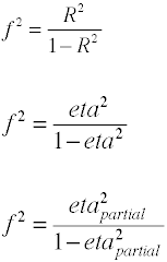
For OLS regression the measure of effects size is F which is defined by Cohen as follows.
Once again there are several ways in which the effect size can be computed from sample data. Note that η2 is another name for R2.
Effect size for F-ratios in analysis of variance
The effect size used in analysis of variance is defined by the ratio of population standard deviations.
Although Cohen’s f is defined as above it is usually computed by taking the square root of f2.
Effect size for χ2 from contingency tables
Once again we start off with the definitional formula in terms of population values. Effect size w is the square root of the standardized chi-square statistic.
And here is how w is computed using sample data.
Here is a table of suggested values for low, medium and high effects (Cohen, 1988). These values should not be taken as absolutes and should interpreted within the context of your research program. The values for large effects are frequently exceeded in practice with values Cohen’s d greater than 1.0 not uncommon. However, using very large effect sizes in prospective power analysis is probably not a good idea as it could lead to under powered studies.
                           small   medum   large
t-test for means      d     .20     .50     .80
t-test for corr       r     .10     .30     .50
F-test for regress    f2    .02     .15     .35
F-test for anova      f     .10     .25     .40
chi-square            w     .10     .30     .50
Comparable effect sizes when there are two groups
        d          r         r2          f         f2
        2       .707    .499849   .9996981   .9993963
      1.9       .689    .474721   .9506578   .9037502
      1.8       .669    .447561   .9000859   .8101547
      1.7       .648    .419904   .8507953   .7238526
      1.6       .625    .390625   .8006408   .6410257
      1.5         .6        .36   .7500001   .5625001
      1.4       .573    .328329   .6991596   .4888242
      1.3       .545    .297025   .6500198   .4225257
      1.2       .514    .264196   .5992141   .3590576
      1.1       .482    .232324   .5501208   .3026329
        1       .447    .199809   .4997016   .2497016
       .9        .41      .1681   .4495192   .2020676
       .8       .371    .137641    .399512   .1596099
       .7        .33      .1089   .3495834   .1222085
       .6       .287    .082369   .2996042   .0897627
       .5       .243    .059049   .2505087   .0627546
       .4       .196    .038416   .1998768   .0399507
       .3       .148    .021904    .149648   .0223945
       .2         .1        .01   .1005038    .010101
       .1        .05      .0025   .0500626   .0025063
        0          0          0          0          0
Some conversion formulas
Convert d to f2
where k = number of groups
Convert t to d for two independent groups
Convert r to d for two independent groups
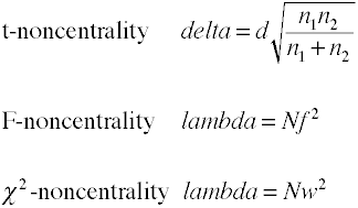
Noncentrality estimates
Power analysis using analytic methods require an estimate of noncentrality which is basically the effect size multiplied by a sample size factor. Here are some formulas for estimating noncentrality.
Example power analysis
Here is an example that brings together effect size and noncentrality in a power analysis.
Consider a one-way analysis of variance with three groups (k = 3). If we expect and
eta2 to equal .12 in which case the effect size will be
effect size f = sqrt(eta2/(1-eta2)) = sqrt(.12/(1-.12)) = .369
With a projected sample size of 60 the estimate of noncentrality is
noncentrality coefficient lambda = N*f = 60*.369^2 = 60*.136 = 8.17
The numerator degrees of freedom is k-1 = 3-1 = 2 while the denominator df is N-k = 60-3 = 57.
The critical value of F with 2 and 57 degrees of freedom is 3.16. Which results in a power of
power = noncentralFtail(df1,df2,lambda,Fcrit(2,57)) = noncentralFtail(2,57,8.17,3.16) = .703
thus, an N of 60 and effect size of .369 yields a projected power of about .7.
We can improve on the power of .7 by using a projected sample size of 75 instead of 60. With the same effect size of .369, we get a new noncentrality estimate of
noncentrality coefficient lambda = N*f = 75*.369^2 = 75*.136 = 10.2
The numerator degrees of freedom remain the same while the denominator df now equal N-k = 75-3 = 72. The critical value of F with 2 and 72 degrees of freedom of 3.12. This time the power is
power = noncentralFtail(df1,df2,lambda,Fcrit(2,72)) = noncentralFtail(2,72,10.2,3.12) = .807
which is within acceptable research limits.
Please note that different stat packages use different names and a different order of
arguments in
the function that we have call noncentralFtail. You will need to read the documentation that
comes with your software.
References
Buchner,A., Erdfelder,E. and Faul,F. How to use G*power. Viewed 19 Jun 2009 <http://www.psycho.uni-duesseldorf.de/aap/projects/gpower/how_to_use_gpower.html>
Becker, L. Psychology 590 course notes. Viewed 19 Jun 2009 <http://web.uccs.edu/lbecker/Psy590/es.htm>
Cohen, J. 1988. Statistical power analysis for the behavioral sciences. Hillsdale, New Jersey: Lawrence Erlbaum Associates


