FAQ: What’s with the different formulas for kurtosis?

In describing the shape statistical distributions kurtosis refers to the “tailedness” of a distribution.

Different statistical packages compute somewhat different values for kurtosis. What are the different formulas used and which packages use which formula?

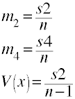
We will begin by defining two different sums of powered deviation scores. The first one, s2, is the sum of squared deviation scores while s4 is the sum of deviation scores raised to the fourth power.

Next, we will define m₂ to be the second moment about the mean of x and m₄ to be the fourth moment. Additionally, V(x) will be the unbiased estimate of the population variance.

Now we can go ahead and start looking at some formulas for kurtosis. The first formula is one that can be found in many statistics books including Snedecor and Cochran (1967). It is used by SAS in proc means when specifying the option vardef=n. This formula is the one most commonly found in general statistics texts. With this definition a perfect normal distribution would have a kurtosis of zero.

The second formula is the one used by Stata with the summarize command. This definition of kurtosis can be found in Bock (1975). The only difference between formula 1 and formula 2 is the -3 in formula 1. Thus, with this formula a perfect normal distribution would have a kurtosis of three.

The third formula, below, can be found in Sheskin (2000) and is used by SPSS and SAS proc means when specifying the option vardef=df or by default if the vardef option is omitted. This formula uses the unbiased estimates of variance and of the fourth moment about the mean. The expected value for kurtosis with a normal distribution is zero.

Examples

Formula 1 — SAS

data test;
  input x;
cards;
1987 
1987 
1991 
1992 
1992 
1992 
1992 
1993 
1994 
1994 
1995 
;
run;

proc means data=test kurtosis vardef=n;
run;

Analysis Variable : x

    Kurtosis
--------------
  -0.2320107
--------------

Formula 2 — Stata

input x
1987
1987
1991
1992
1992
1992
1992
1993
1994
1994
1995
end

summ x, detail
                              x
-------------------------------------------------------------
      Percentiles      Smallest
 1%         1987           1987
 5%         1987           1987
10%         1987           1991       Obs                  11
25%         1991           1992       Sum of Wgt.          11

50%         1992                      Mean           1991.727
                        Largest       Std. Dev.      2.611165
75%         1994           1993
90%         1994           1994       Variance       6.818182
95%         1995           1994       Skewness      -.8895014
99%         1995           1995       Kurtosis       2.767989

Formula 3 — SAS

data test;
  input x;
cards;
1987 
1987 
1991 
1992 
1992 
1992 
1992 
1993 
1994 
1994 
1995 
;
run;

proc means data=test kurtosis vardef=df;
run;

Analysis Variable : x

    Kurtosis
--------------
   0.4466489
--------------

proc means data=test kurtosis;
run;

Analysis Variable : x

    Kurtosis
--------------
   0.4466489
--------------

Formula 3 — SPSS

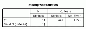
data list list / yr.
begin data.
1987 
1987 
1991 
1992 
1992 
1992 
1992 
1993 
1994 
1994 
1995 
end data.

desc /var=all /stat=kurtosis.

References

Bock, R.D. (1975) Multivariate Statistical Methods in Behavioral Research. New York: McGraw-Hill.

Joanest, D.N. and Gill, C.A. (1998) Comparing measures of sample skewness and kurtosis. The Statistician, 47, pp 183-189.

Sheskin, D.J. (2000) Handbook of Parametric and Nonparametric Statistical Procedures, Second Edition. Boca Raton, Florida: Chapman & Hall/CRC.

Snedecor, G.W. and Cochran, W.G. (1967) Statistical Methods, Sixth Edition. Ames, Iowa: Iowa State University Press.

Westfall, P. (2014) Kurtosis as Peakedness, 1905 – 2014. R.I.P. American Statistician, 68(3): 191-195.