When I run my OLS regression model with a constant I get an R2 of about 0.35 and an F-ratio around 100. When I run the same model without a constant the R2 is 0.97 and the F-ratio is over 7,000. Why are R2 and F-ratio so large for models without a constant?
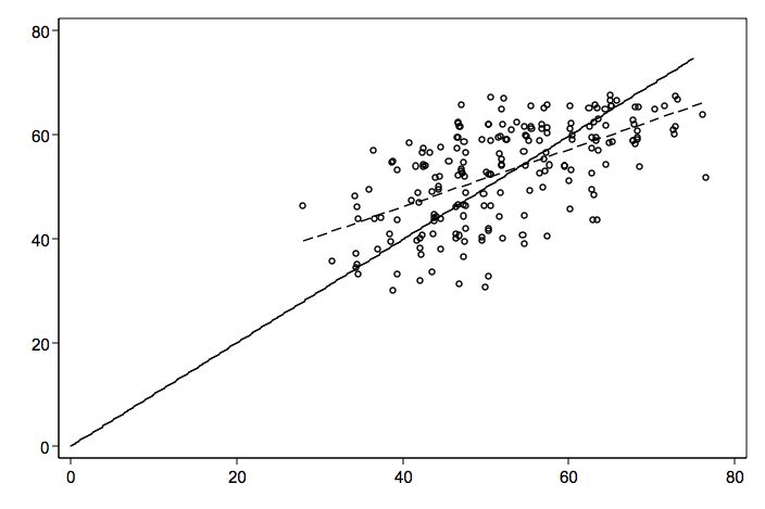
Let’s begin by going over what it means to run an OLS regression without a constant (intercept). A regression without a constant implies that the regression line should run through the origin, i.e., the point where both the response variable and predictor variable equal zero. Let’s look at a scatterplot that has both the regular regression line (dashed line) and a line without the constant (solid line).
As you can see, the “true” regression line is different from noconstant line. Then how can it be that the noconstant model has a larger R2 and F-ratio then a model with a constant?
To answer this question, let’s start with a review how the R2 and F-ratio for OLS regression models
are computed.
[
R^{2} = frac{SS_{model}}{SS_{model} + SS_{residual}}
]
[
F = frac{left(frac{SS_{model}}{df_{model}}right)}{left(frac{SS_{residual}}{df_{residual}}right)}
]
Next, let’s see how each of these sums of squares are defined. For these equations we will use (hat{Y}) for the predicted value of the response variable Y and (bar{Y}) for the mean value of Y. [ SS_{total} = sum_{i = 1}^{N}(Y_i – bar{Y})^2 ] [ SS_{model} = sum_{i = 1}^{N}(hat{Y}_i – bar{Y})^2 ] [ SS_{residual} = sum_{i = 1}^{N}(Y_i – hat{Y}_i)^2 ]
When you run the regression without a constant in the model, you are declaring that the expected value of Y when x is equal to 0 is 0. That is, (E(Y | x = 0) = 0). If this is not the case, the values of (hat{Y}) will be different yielding different (SS_{model}) and (SS_{residual}) hence different (R^2) and F values. Typically, the sum of squares of Y accounted for by the intercept are not included in the total sum of squares. That is, they are neither in SSmodel nor SSresidual. That is the model is predicting the sum of squares left over after taking out the intercept. When the intercept (or constant term) is left off and it does not have a true zero effect, the total sum of squares being modelled is increased. This tends to inflate both SSmodel and SSresidual; however, SSmodel increases relatively more than SSresidual leading to the increase in R2 values.
The actual code used to calculate (R^2) are different with and without an intercept. This is easy to see by running models without a built-in intercept, but manually including one (a constant term). Here is some example code you can try:
sysuse auto
gen const = 1
regress mpg weight
      Source |       SS       df       MS              Number of obs =      74
-------------+------------------------------           F(  1,    72) =  134.62
       Model |   1591.9902     1   1591.9902           Prob > F      =  0.0000
    Residual |  851.469256    72  11.8259619           R-squared     =  0.6515
-------------+------------------------------           Adj R-squared =  0.6467
       Total |  2443.45946    73  33.4720474           Root MSE      =  3.4389

------------------------------------------------------------------------------
         mpg |      Coef.   Std. Err.      t    P>|t|     [95% Conf. Interval]
-------------+----------------------------------------------------------------
      weight |  -.0060087   .0005179   -11.60   0.000    -.0070411   -.0049763
       _cons |   39.44028   1.614003    24.44   0.000     36.22283    42.65774
------------------------------------------------------------------------------
regress mpg const weight, noconstant
      Source |       SS       df       MS              Number of obs =      74
-------------+------------------------------           F(  2,    72) = 1486.41
       Model |  35156.5307     2  17578.2654           Prob > F      =  0.0000
    Residual |  851.469256    72  11.8259619           R-squared     =  0.9764
-------------+------------------------------           Adj R-squared =  0.9757
       Total |       36008    74  486.594595           Root MSE      =  3.4389

------------------------------------------------------------------------------
         mpg |      Coef.   Std. Err.      t    P>|t|     [95% Conf. Interval]
-------------+----------------------------------------------------------------
       const |   39.44028   1.614003    24.44   0.000     36.22283    42.65774
      weight |  -.0060087   .0005179   -11.60   0.000    -.0070411   -.0049763
------------------------------------------------------------------------------
regress mpg weight, noconstant
* note change in total SS between plain regress and wihtout constant
* but total SS is the same for without constant and with const
* when using manual intercept, intercept SS included in model
      Source |       SS       df       MS              Number of obs =      74
-------------+------------------------------           F(  1,    73) =  259.18
       Model |  28094.8545     1  28094.8545           Prob > F      =  0.0000
    Residual |  7913.14549    73  108.399253           R-squared     =  0.7802
-------------+------------------------------           Adj R-squared =  0.7772
       Total |       36008    74  486.594595           Root MSE      =  10.411

------------------------------------------------------------------------------
         mpg |      Coef.   Std. Err.      t    P>|t|     [95% Conf. Interval]
-------------+----------------------------------------------------------------
      weight |    .006252   .0003883    16.10   0.000     .0054781     .007026
------------------------------------------------------------------------------
one <- rep(1, 32)
anova(lm(mpg ~ qsec, data = mtcars))
Analysis of Variance Table

Response: mpg
          Df Sum Sq Mean Sq F value  Pr(>F)
qsec       1 197.39 197.392  6.3767 0.01708 *
Residuals 30 928.66  30.955
---
Signif. codes:  0 '***' 0.001 '**' 0.01 '*' 0.05 '.' 0.1 ' ' 1
anova(lm(mpg ~ 0 + one + qsec, data = mtcars))
Analysis of Variance Table

Response: mpg
          Df  Sum Sq Mean Sq  F value  Pr(>F)
one        1 12916.3 12916.3 417.2570 < 2e-16 ***
qsec       1   197.4   197.4   6.3767 0.01708 *
Residuals 30   928.7    31.0
---
Signif. codes:  0 '***' 0.001 '**' 0.01 '*' 0.05 '.' 0.1 ' ' 1
anova(lm(mpg ~ 0 + qsec, data = mtcars))
Analysis of Variance Table

Response: mpg
          Df  Sum Sq Mean Sq F value    Pr(>F)
qsec       1 13105.6 13105.6  433.73 < 2.2e-16 ***
Residuals 31   936.7    30.2
---
Signif. codes:  0 '***' 0.001 '**' 0.01 '*' 0.05 '.' 0.1 ' ' 1

