Consider the six graphs of the nonlinear (curvilinear) relationships depicted below.
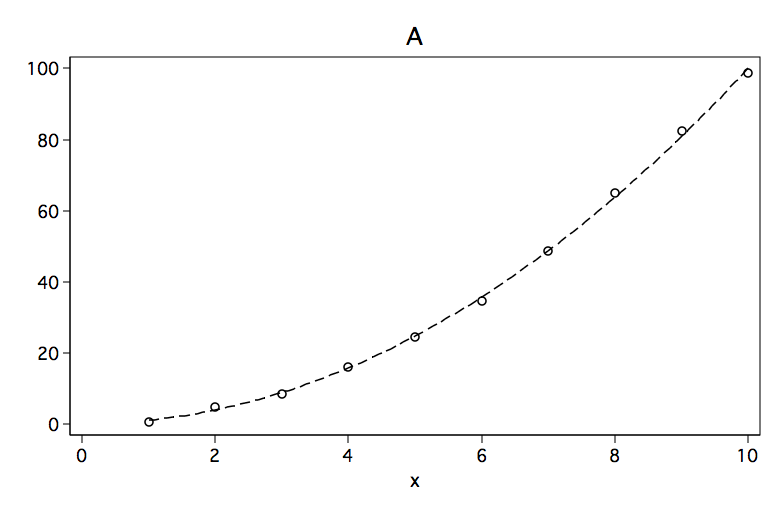
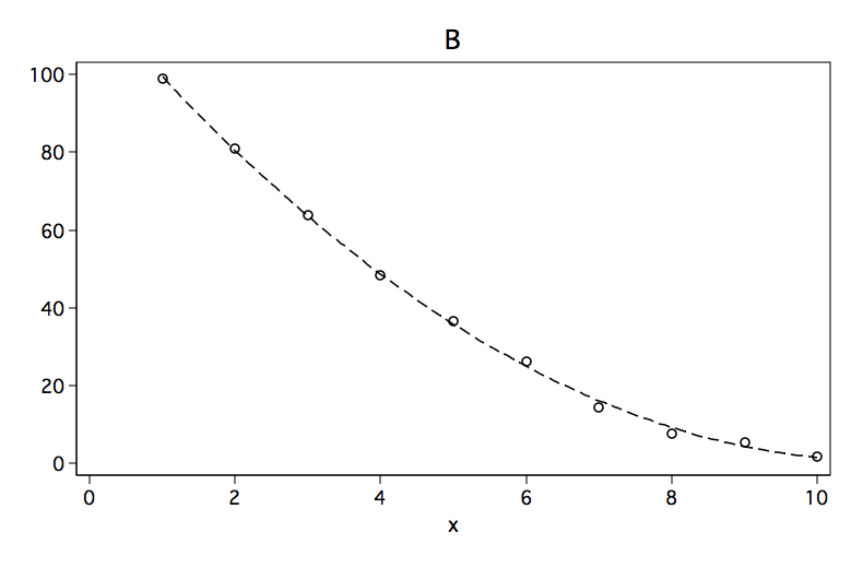
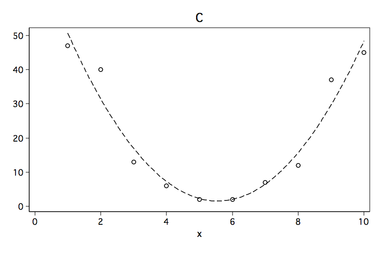
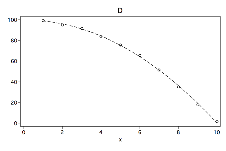
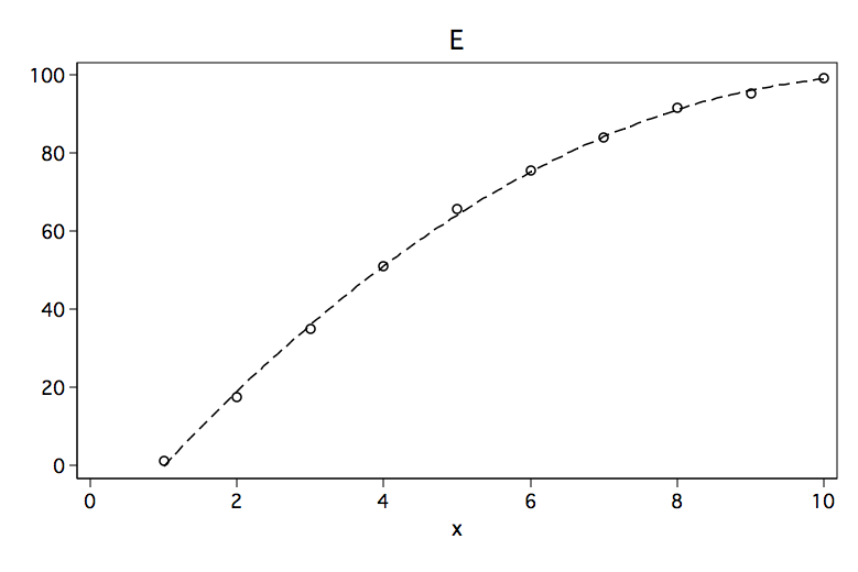
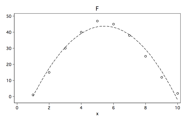
Although each of the six figures look like very different curves, there are some similarities. For example, curves A, B and C would be considered to be convex (apex at the bottom, curve opens up) while curves D, E and F are concave (apex at the top, curve opens down).
Below are the results of fitting a polynomial regression model to data points for each of the six figures. The predictors in the model are x and x2 where x2 is x^2. Please note the sign for x2 in each of the models. The sign is positive when the model is convex and negative when the curve is concave.
------------------------------------------------------------------------------
     Model A |      Coef.   Std. Err.      t    P>|t|     [95% Conf. Interval]
-------------+----------------------------------------------------------------
           x |  -.1839751   .5230228    -0.35   0.735    -1.420728    1.052777
          x2 |   1.016747   .0463379    21.94   0.000     .9071754    1.126319
    constant |   .2076584   1.252323     0.17   0.873    -2.753615    3.168931
------------------------------------------------------------------------------

------------------------------------------------------------------------------
     Model B |      Coef.   Std. Err.      t    P>|t|     [95% Conf. Interval]
-------------+----------------------------------------------------------------
           x |  -21.93563    .550781   -39.83   0.000    -23.23802   -20.63324
          x2 |   1.003714   .0487971    20.57   0.000     .8883275    1.119101
    constant |   120.3872   1.318787    91.29   0.000     117.2688    123.5057
------------------------------------------------------------------------------

------------------------------------------------------------------------------
     Model C |      Coef.   Std. Err.      t    P>|t|     [95% Conf. Interval]
-------------+----------------------------------------------------------------
           x |  -26.33182   2.511897   -10.48   0.000    -32.27151   -20.39213
          x2 |   2.371212   .2225446    10.65   0.000     1.844978    2.897447
    constant |   74.63333   6.014471    12.41   0.000     60.41137     88.8553
------------------------------------------------------------------------------

------------------------------------------------------------------------------
     Model D |      Coef.   Std. Err.      t    P>|t|     [95% Conf. Interval]
-------------+----------------------------------------------------------------
           x |   .1839751   .5230227     0.35   0.735    -1.052777    1.420727
          x2 |  -1.016747   .0463378   -21.94   0.000    -1.126319   -.9071754
    constant |   99.79234   1.252322    79.69   0.000     96.83107    102.7536
------------------------------------------------------------------------------

------------------------------------------------------------------------------
     Model E |      Coef.   Std. Err.      t    P>|t|     [95% Conf. Interval]
-------------+----------------------------------------------------------------
           x |      22.15   .5390466    41.09   0.000     20.87536    23.42464
          x2 |  -1.012121   .0477575   -21.19   0.000     -1.12505   -.8991926
    constant |  -21.27333    1.29069   -16.48   0.000    -24.32533   -18.22133
------------------------------------------------------------------------------

------------------------------------------------------------------------------
     Model F |      Coef.   Std. Err.      t    P>|t|     [95% Conf. Interval]
-------------+----------------------------------------------------------------
           x |   24.10227   1.615884    14.92   0.000     20.28132    27.92323
          x2 |  -2.215909   .1431612   -15.48   0.000    -2.554432   -1.877387
    constant |     -21.75   3.869062    -5.62   0.001    -30.89888   -12.60112
------------------------------------------------------------------------------
Okay, so the quadratic term, x2, indicates which way the curve is bending but what’s up with the linear term, x, it doesn’t seem to make sense. The explanation for this will require a bit of math but the solution is actually rather easy. Let’s look at the linear model.
- y = b0 + b1*x + b2*x2
If we differentiate with respect to x we get,
- y’ = b1 + 2*b2*x.
What this shows is that b1 gives the rate of change when x is equal to zero. In our example above x = 0 is not within range of our observed values. The coefficient b2 tells both the direction and steepness of the curvature (a positive value indicates the curvature is upwards while a negative value indicates the curvature is downwards).
So the trick is to place the zero value within the range of our data. We will do this by centering the x, that is, we will subtract the mean of x from each value. We will call this new variable c and we will then create c2 by squaring c. Next, we will rerun the four regression models. You note that the coefficient for the quadratic term are unchanged while the coefficient for the linear better reflect the linear relation, which in the case of Models C and F should be somewhat near zero.
------------------------------------------------------------------------------
    Model A  |      Coef.   Std. Err.      t    P>|t|     [95% Conf. Interval]
-------------+----------------------------------------------------------------
           c |   11.00024   .1172265    93.84   0.000     10.72304    11.27744
          c2 |   1.016747   .0463379    21.94   0.000     .9071754    1.126319
    constant |   29.95239   .5094267    58.80   0.000     28.74779    31.15699
------------------------------------------------------------------------------

------------------------------------------------------------------------------
    Model B  |      Coef.   Std. Err.      t    P>|t|     [95% Conf. Interval]
-------------+----------------------------------------------------------------
           c |  -10.89477    .123448   -88.25   0.000    -11.18668   -10.60286
          c2 |   1.003714   .0487971    20.57   0.000     .8883275    1.119101
    constant |   30.10364   .5364633    56.12   0.000     28.83511    31.37218
------------------------------------------------------------------------------

------------------------------------------------------------------------------
    Model C  |      Coef.   Std. Err.      t    P>|t|     [95% Conf. Interval]
-------------+----------------------------------------------------------------
           c |  -.2484848   .5629983    -0.44   0.672    -1.579764    1.082795
          c2 |   2.371212   .2225446    10.65   0.000     1.844978    2.897447
    constant |     1.5375   2.446599     0.63   0.550    -4.247788    7.322788
------------------------------------------------------------------------------

------------------------------------------------------------------------------
    Model D  |      Coef.   Std. Err.      t    P>|t|     [95% Conf. Interval]
-------------+----------------------------------------------------------------
           c |  -11.00024   .1172265   -93.84   0.000    -11.27744   -10.72304
          c2 |  -1.016747   .0463378   -21.94   0.000    -1.126319   -.9071754
    constant |   70.04761   .5094266   137.50   0.000     68.84301    71.25221
------------------------------------------------------------------------------

------------------------------------------------------------------------------
    Model E  |      Coef.   Std. Err.      t    P>|t|     [95% Conf. Interval]
-------------+----------------------------------------------------------------
           c |   11.01667    .120818    91.18   0.000     10.73098    11.30236
          c2 |  -1.012121   .0477575   -21.19   0.000     -1.12505   -.8991926
    constant |     69.935    .525034   133.20   0.000     68.69349    71.17651
------------------------------------------------------------------------------

------------------------------------------------------------------------------
    Model F  |      Coef.   Std. Err.      t    P>|t|     [95% Conf. Interval]
-------------+----------------------------------------------------------------
           c |  -.2727273   .3621724    -0.75   0.476    -1.129129    .5836743
          c2 |  -2.215909   .1431612   -15.48   0.000    -2.554432   -1.877387
    constant |   43.78125   1.573878    27.82   0.000     40.05962    47.50288
------------------------------------------------------------------------------
As an added benefit centering the x variable reduces the correlation between the linear and quadratic terms. The correlation between x and x2 is 0.975 while the correlation between c and c2 is 0.000.