When you conduct a test of statistical significance, whether it is from a correlation, an ANOVA, regression or some other kind of test, you are given a p-value somewhere in the output. Unless you specify otherwise, this p-value (almost always) is for a two-tailed test. But what does this mean, really, and how can you convert this into a one-tailed test?
What is a two-tailed test?
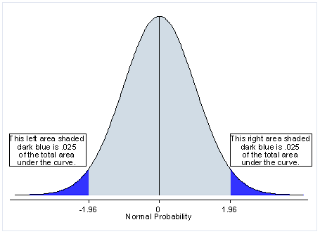
First let’s start with the meaning of a two-tailed test. If you are using a significance level of .05, a two-tailed test divides this value in half, meaning that .025 is in each tail of the distribution. While this makes it more difficult to achieve statistical significance, this means that you do not have make a prediction about the direction of the effect. In other words, the effect can be either positive or negative and still be statistically significant.
Converting a two-tailed to a one-tailed test
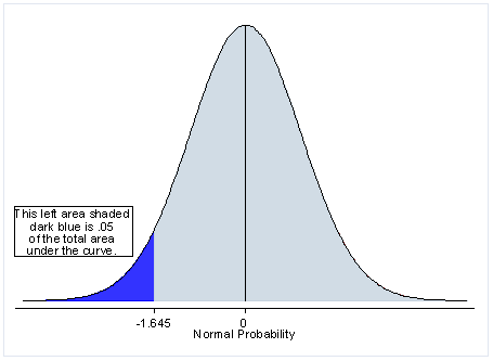
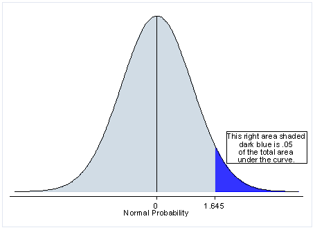
The easiest way to convert a two-tailed test into a one-tailed test is to divide in half the p-value provided in the output. In the output below, under the headings Ha: diff < 0 and Ha: diff > 0 are the results for the one-tailed tests, and the results in the middle, under the heading Ha: diff != 0 (which means that the difference is not equal to 0), is the two-tailed test. We can look at the output below and see that this is done to create the appropriate p-value for the predicted direction (see bolded portion). Notice, though, that there is no way to get a statistically significant result in the other direction. You need to make the directional prediction before you conduct the test, and if the result goes in the opposite direction, even if it would have been statistically significant with a two-tailed test, it is not statistically significant. To report the p-value in this direction, you would take the p-value from the one-tailed test and subtract that from 1. You can see this in the example below, 1 – .0001 = .9999.
Two-sample t test with equal variances

------------------------------------------------------------------------------
   Group |     Obs        Mean    Std. Err.   Std. Dev.   [95% Conf. Interval]
---------+--------------------------------------------------------------------
    male |      91    50.12088    1.080274    10.30516    47.97473    52.26703
  female |     109    54.99083    .7790686    8.133715    53.44658    56.53507
---------+--------------------------------------------------------------------
combined |     200      52.775    .6702372    9.478586    51.45332    54.09668
---------+--------------------------------------------------------------------
    diff |           -4.869947    1.304191               -7.441835   -2.298059
------------------------------------------------------------------------------
Degrees of freedom: 198
                  Ho: mean(male) - mean(female) = diff = 0
     Ha: diff < 0               Ha: diff != 0              Ha: diff > 0
       t =  -3.7341                t =  -3.7341              t =  -3.7341
   P < t =   0.0001          P > |t| =   0.0002          P > t =   0.9999
One-tailed test distribution
Why would you use a one-tailed test?
Many researchers argue that it is very rarely appropriate to do a one-tailed test. However, if it is logically impossible for the result to go in one direction (for example, for the mean height of 5-year-olds to be smaller than the mean height of 15-year-olds) or if such a result is of no practical importance (for example, the experimental medicine is less effective than currently used medicine), then a one-tailed test is appropriate. Also note that a one-tailed test has more power than a two-tailed test. In other words, while the probability of a Type I error is the same (whatever alpha level is used), the probability of a Type II error is reduced. Hence, you are less likely to miss a statistically significant effect with a one-tailed test (assuming that you have accurately predicted the direction of the effect).
Another example
Now let’s try an example using a regression analysis. Let’s say that we have social studies, math and science test scores from high school students and that we predict that the science scores will positively predict the social studies scores. In other words, we want to conduct a one-tailed test, and we will be using the distribution immediately above. Below is the output.
      Source |       SS       df       MS              Number of obs =     200
-------------+------------------------------           F(  2,   197) =   46.58
       Model |  7363.62077     2  3681.81039           Prob > F      =  0.0000
    Residual |  15572.5742   197  79.0486001           R-squared     =  0.3210
-------------+------------------------------           Adj R-squared =  0.3142
       Total |   22936.195   199  115.257261           Root MSE      =  8.8909
------------------------------------------------------------------------------
       socst |      Coef.   Std. Err.      t    P>|t|     [95% Conf. Interval]
-------------+----------------------------------------------------------------
     science |   .2191144   .0820323     2.67   0.008     .0573403    .3808885
        math |   .4778911   .0866945     5.51   0.000     .3069228    .6488594
       _cons |   15.88534   3.850786     4.13   0.000     8.291287    23.47939
------------------------------------------------------------------------------
To get the p-value for the one-tailed test of the variable science (assuming that the effect is going in the predicted direction, which you can tell by the sign of the coefficient), you would divide the .008 by 2, yielding .004. If you had made your prediction in the opposite direction, the p-value would have been 1 – .004 = .996.


