Introduction to Generalized Linear Mixed Models

Background

Generalized linear mixed models (or GLMMs) are an extension of linear mixed models to allow response variables from different distributions, such as binary responses. Alternatively, you could think of GLMMs as an extension of generalized linear models (e.g., logistic regression) to include both fixed and random effects (hence mixed models). The general form of the model (in matrix notation) is:

$$\mathbf{y}=\mathbf{X}\mathit{\beta }+\mathbf{Z}\mathbf{u}+\mathit{\epsilon }$$

Where $\mathbf{y}$ is a $N\times 1$ column vector, the outcome variable; $\mathbf{X}$ is a $N\times p$ matrix of the $p$ predictor variables; $\mathit{\beta }$ is a $p\times 1$ column vector of the fixed-effects regression coefficients (the $\beta$s); $\mathbf{Z}$ is the $N\times q$ design matrix for the $q$ random effects (the random complement to the fixed $\mathbf{X})$; $\mathbf{u}$ is a $q\times 1$ vector of the random effects (the random complement to the fixed $\mathit{\beta })$; and $\mathit{\epsilon }$ is a $N\times 1$ column vector of the residuals, that part of $\mathbf{y}$ that is not explained by the model, $\mathit{X}\mathit{\beta }+\mathbf{Zu}$. To recap:

$$\stackrel{\text{N x 1}}{\overbrace{\mathbf{y}}}=\stackrel{\text{N x 1}}{\overbrace{\underset{\text{N x p}}{\underbrace{\mathbf{X}}}\underset{\text{p x 1}}{\underbrace{\mathit{\beta }}}}}+\stackrel{\text{N x 1}}{\overbrace{\underset{\text{N x q}}{\underbrace{\mathbf{Z}}}\underset{\text{q x 1}}{\underbrace{\mathbf{u}}}}}+\stackrel{\text{N x 1}}{\overbrace{\mathit{\epsilon }}}$$

To make this more concrete, let’s consider an example from a simulated dataset. Doctors ($q=407$) indexed by the $j$ subscript each see $n_j$ patients. So our grouping variable is the doctor. Not every doctor sees the same number of patients, ranging from just 2 patients all the way to 40 patients, averaging about 21. The total number of patients is the sum of the patients seen by each doctor

$$N=\sum _j^q{n}_j$$

In our example, $N=8525$ patients were seen by doctors. Our outcome, $\mathbf{y}$ is a continuous variable, mobility scores. Further, suppose we had 6 fixed effects predictors, Age (in years), Married (0 = no, 1 = yes), Sex (0 = female, 1 = male), Red Blood Cell (RBC) count, and White Blood Cell (WBC) count plus a fixed intercept and random intercept for every doctor. For simplicity, we are only going to consider random intercepts. We will let every other effect be fixed for now. The reason we want any random effects is because we expect that mobility scores within doctors may be correlated. There are many reasons why this could be. For example, doctors may have specialties that mean they tend to see lung cancer patients with particular symptoms or some doctors may see more advanced cases, such that within a doctor, patients are more homogeneous than they are between doctors. To put this example back in our matrix notation, we would have:

$$\stackrel{\text{8525 x 1}}{\overbrace{\mathbf{y}}}=\stackrel{\text{8525 x 1}}{\overbrace{\underset{\text{8525 x 6}}{\underbrace{\mathbf{X}}}\underset{\text{6 x 1}}{\underbrace{\mathit{\beta }}}}}+\stackrel{\text{8525 x 1}}{\overbrace{\underset{\text{8525 x 407}}{\underbrace{\mathbf{Z}}}\underset{\text{407 x 1}}{\underbrace{\mathbf{u}}}}}+\stackrel{\text{8525 x 1}}{\overbrace{\mathit{\epsilon }}}$$

$$\mathbf{y}=\left[\begin{array}{l}\text{mobility}\\ 2\\ 2\\ \dots \\ 3\end{array}\right]\begin{array}{l}{n}_{ij}\\ 1\\ 2\\ \dots \\ 8525\end{array}\mathbf{X}=\left[\begin{array}{llllll}\text{Intercept}& \text{Age}& \text{Married}& \text{Sex}& \text{WBC}& \text{RBC}\\ 1& 64.97& 0& 1& 6087& 4.87\\ 1& 53.92& 0& 0& 6700& 4.68\\ \dots & \dots & \dots & \dots & \dots & \dots \\ 1& 56.07& 0& 1& 6430& 4.73\end{array}\right]$$

$$\mathit{\beta }=\left[\begin{array}{c}4.782\\ .025\\ .011\\ .012\\ 0\\ -.009\end{array}\right]$$

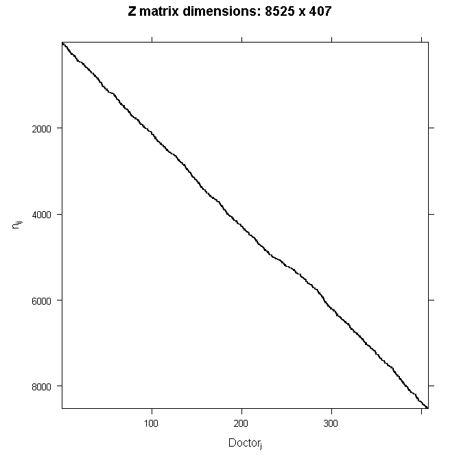
Because $\mathbf{Z}$ is so big, we will not write out the numbers here. Because we are only modeling random intercepts, it is a special matrix in our case that only codes which doctor a patient belongs to. So in this case, it is all 0s and 1s. Each column is one doctor and each row represents one patient (one row in the dataset). If the patient belongs to the doctor in that column, the cell will have a 1, 0 otherwise. This also means that it is a sparse matrix (i.e., a matrix of mostly zeros) and we can create a picture representation easily. Note that if we added a random slope, the number of rows in $\mathbf{Z}$ would remain the same, but the number of columns would double. This is why it can become computationally burdensome to add random effects, particularly when you have a lot of groups (we have 407 doctors). In all cases, the matrix will contain mostly zeros, so it is always sparse. In the graphical representation, the line appears to wiggle because the number of patients per doctor varies.

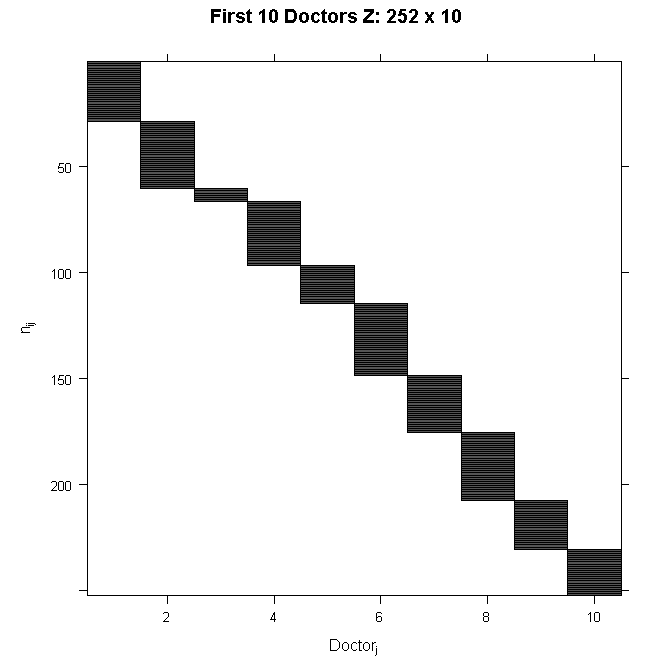
In order to see the structure in more detail, we could also zoom in on just the first 10 doctors. The filled space indicates rows of observations belonging to the doctor in that column, whereas the white space indicates not belonging to the doctor in that column.

If we estimated it, $\mathbf{u}$ would be a column vector, similar to $\mathit{\beta }$. However, in classical statistics, we do not actually estimate $\mathbf{u}$. Instead, we nearly always assume that for the $j$ th element of vector $\mathbf{u}$:

$$u_j\sim \mathcal{N}(\mathbf{0},\mathbf{G})$$

Which is read: “$u_j$ is distributed as normal with mean zero and variance G”. Where $\mathbf{G}$ is the variance-covariance matrix of the random effects. Because we directly estimated the fixed effects, including the fixed effect intercept, random effect complements are modeled as deviations from the fixed effect, so they have mean zero. The random effects are just deviations around the value in $\mathit{\beta }$, which is the mean. So what is left to estimate is the variance. Because our example only had a random intercept, $\mathbf{G}$ is just a $1\times 1$ matrix, the variance of the random intercept. However, it can be larger. For example, suppose that we had a random intercept and a random slope, then

$$\mathbf{G}=\left[\begin{array}{cc}{\sigma }_{int}^2& {\sigma }_{int,slope}^2\\ {\sigma }_{int,slope}^2& {\sigma }_{slope}^2\end{array}\right]$$

Because $\mathbf{G}$ is a variance-covariance matrix, we know that it should have certain properties. In particular, we know that it is square, symmetric, and positive semidefinite. We also know that this matrix has redundant elements. For a $q\times q$ matrix, there are $\frac{q(q+1)}{2}$ unique elements. To simplify computation by removing redundant effects and ensure that the resulting estimate matrix is positive definite, rather than model $\mathbf{G}$ directly, we estimate $\mathit{\theta }$ (e.g., a triangular Cholesky factorization $\mathbf{G}={\mathbf{LDL}}^{\mathbf{T}}$). $\mathit{\theta }$ is not always parameterized the same way, but you can generally think of it as representing the random effects. It is usually designed to contain non redundant elements (unlike the variance covariance matrix) and to be parameterized in a way that yields more stable estimates than variances (such as taking the natural logarithm to ensure that the variances are positive). Regardless of the specifics, we can say that

$$\mathbf{G}=\sigma (\mathit{\theta })$$

In other words, $\mathbf{G}$ is some function of $\mathit{\theta }$. So we get some estimate of $\mathit{\theta }$ which we call $\hat{\mathit{\theta }}$. Various parameterizations and constraints allow us to simplify the model for example by assuming that the random effects are independent, which would imply the true structure is

$$\mathbf{G}=\left[\begin{array}{cc}{\sigma }_{int}^2& 0\\ 0& {\sigma }_{slope}^2\end{array}\right]$$

The final element in our model is the variance-covariance matrix of the residuals, $\epsilon$ or the conditional covariance matrix of $\mathbf{y}|\mathit{X}\mathit{\beta }+\mathit{Z}\mathit{u}$. The most common residual covariance structure is

$$\mathbf{R}=\mathit{I}{\mathit{\sigma }}_{\mathit{\epsilon }}^{\mathbf{2}}$$

where $\mathbf{I}$ is the identity matrix (diagonal matrix of 1s) and ${\sigma }_{\epsilon }^2$ is the residual variance. This structure assumes a homogeneous residual variance for all (conditional) observations and that they are (conditionally) independent. Other structures can be assumed such as compound symmetry or autoregressive. The $\mathbf{G}$ terminology is common in SAS, and also leads to talking about G-side structures for the variance covariance matrix of random effects and R-side structures for the residual variance covariance matrix.

So the final fixed elements are $\mathbf{y}$, $\mathbf{X}$, $\mathbf{Z}$, and $\mathit{\epsilon }$. The final estimated elements are $\hat{\mathit{\beta }}$, $\hat{\mathit{\theta }}$, $\hat{\mathbf{G}}$, and $\hat{\mathbf{R}}$. The final model depends on the distribution assumed, but is generally of the form:

$$\mathbf{y}|\mathit{X}\mathit{\beta }+\mathit{Z}\mathit{u}\sim \mathcal{F}(\mathbf{0},\mathbf{R})$$

We could also frame our model in a two level-style equation for the $i$-th patient for the $j$-th doctor. There we are working with variables that we subscript rather than vectors as before. The level 1 equation adds subscripts to the parameters $\beta$s to indicate which doctor they belong to. Turning to the level 2 equations, we can see that each $\beta$ estimate for a particular doctor, ${\beta }_{pj}$, can be represented as a combination of a mean estimate for that parameter, ${\gamma }_{p0}$, and a random effect for that doctor, ($u_{pj}$). In this particular model, we see that only the intercept (${\beta }_{0j}$) is allowed to vary across doctors because it is the only equation with a random effect term, ($u_{0j}$). The other ${\beta }_{pj}$ are constant across doctors.

$$\begin{array}{ll}L1:& Y_{ij}={\beta }_{0j}+{\beta }_{1j}Ag{e}_{ij}+{\beta }_{2j}Marrie{d}_{ij}+{\beta }_{3j}Se{x}_{ij}+{\beta }_{4j}WB{C}_{ij}+{\beta }_{5j}RB{C}_{ij}+e_{ij}\\ L2:& {\beta }_{0j}={\gamma }_{00}+u_{0j}\\ L2:& {\beta }_{1j}={\gamma }_{10}\\ L2:& {\beta }_{2j}={\gamma }_{20}\\ L2:& {\beta }_{3j}={\gamma }_{30}\\ L2:& {\beta }_{4j}={\gamma }_{40}\\ L2:& {\beta }_{5j}={\gamma }_{50}\end{array}$$

Substituting in the level 2 equations into level 1, yields the mixed model specification. Here we grouped the fixed and random intercept parameters together to show that combined they give the estimated intercept for a particular doctor.

$$Y_{ij}=({\gamma }_{00}+u_{0j})+{\gamma }_{10}Ag{e}_{ij}+{\gamma }_{20}Marrie{d}_{ij}+{\gamma }_{30}SE{X}_{ij}+{\gamma }_{40}WB{C}_{ij}+{\gamma }_{50}RB{C}_{ij}+e_{ij}$$

Generalized Linear Mixed Models

Up to this point everything we have said applies equally to linear mixed models as to generalized linear mixed models. Now let’s focus in on what makes GLMMs unique.

What is different between LMMs and GLMMs is that the response variables can come from different distributions besides gaussian. In addition, rather than modeling the responses directly, some link function is often applied, such as a log link. We will talk more about this in a minute. Let the linear predictor, $\eta$, be the combination of the fixed and random effects excluding the residuals.

$$\mathit{\eta }=\mathit{X}\mathit{\beta }+\mathit{Z}\mathit{\gamma }$$

The generic link function is called $g(\cdot )$. The link function relates the outcome $\mathbf{y}$ to the linear predictor $\eta$. Thus:

$$\begin{array}{l}\mathit{\eta }=\mathit{X}\mathit{\beta }+\mathit{Z}\mathit{\gamma }\\ g(\cdot )=\text{link function}\\ h(\cdot )=g^{-1}(\cdot )=\text{inverse link function}\end{array}$$

So our model for the conditional expectation of $\mathbf{y}$ (conditional because it is the expected value depending on the level of the predictors) is:

$$g(E(\mathbf{y}))=\mathit{\eta }$$

We could also model the expectation of $\mathbf{y}$:

$$E(\mathbf{y})=h(\mathit{\eta })=\mathit{\mu }$$

With $\mathbf{y}$ itself equal to:

$$\mathbf{y}=h(\mathit{\eta })+\mathit{\epsilon }$$

Link Functions and Families

So what are the different link functions and families? There are many options, but we are going to focus on three, link functions and families for binary outcomes, count outcomes, and then tie it back in to continuous (normally distributed) outcomes.

For a binary outcome, we use a logistic link function and the probability density function, or PDF, for the logistic. These are:

$$\begin{array}{l}g(\cdot )=lo{g}_e(\frac{p}{1–p})\\ h(\cdot )=\frac{e^{(\cdot )}}{1+e^{(\cdot )}}\\ PDF=\frac{e^{-\left(\frac{x–\mu }{s}\right)}}{s{(1+e^{-\left(\frac{x–\mu }{s}\right)})}^2}\\ \text{where }s=1\text{ which is the most common default (scale fixed at 1)}\\ PDF=\frac{e^{-(x–\mu )}}{{(1+e^{-(x–\mu )})}^2}\\ E(X)=\mu \\ Var(X)=\frac{{\pi }^2}{3}\end{array}$$

Count Outcomes

For a count outcome, we use a log link function and the probability mass function, or PMF, for the poisson. Note that we call this a probability mass function rather than probability density function because the support is discrete (i.e., for positive integers). These are:

$$\begin{array}{l}g(\cdot )=lo{g}_e(\cdot )\\ h(\cdot )=e^{(\cdot )}\\ PMF=Pr(X=k)=\frac{{\lambda }^k{e}^{-\lambda }}{k!}\\ E(X)=\lambda \\ Var(X)=\lambda \end{array}$$

Continuous Outcomes

For a continuous outcome where we assume a normal distribution, the most common link function is simply the identity. In this case, there are some special properties that simplify things:

$$\begin{array}{l}g(\cdot )=\cdot \\ h(\cdot )=\cdot \\ g(\cdot )=h(\cdot )\\ g(E(X))=E(X)=\mu \\ g(Var(X))=Var(X)={\mathrm{\Sigma }}^2\\ PDF(X)=\left(\frac{1}{\mathrm{\Sigma }\sqrt{2\pi }}\right)e^{\frac{-(x–\mu {)}^2}{2{\mathrm{\Sigma }}^2}}\end{array}$$

So you can see how when the link function is the identity, it essentially drops out and we are back to our usual specification of means and variances for the normal distribution, which is the model used for typical linear mixed models. Thus generalized linear mixed models can easily accommodate the specific case of linear mixed models, but generalize further.

Interpretation

The interpretation of GLMMs is similar to GLMs; however, there is an added complexity because of the random effects. On the linearized metric (after taking the link function), interpretation continues as usual. However, it is often easier to back transform the results to the original metric. For example, in a random effects logistic model, one might want to talk about the probability of an event given some specific values of the predictors. Likewise in a poisson (count) model, one might want to talk about the expected count rather than the expected log count. These transformations complicate matters because they are nonlinear and so even random intercepts no longer play a strictly additive role and instead can have a multiplicative effect. This section discusses this concept in more detail and shows how one could interpret the model results.

Suppose we estimated a mixed effects logistic model, predicting remission (yes = 1, no = 0) from Age, Married (yes = 1, no = 0), and IL6 (continuous). We allow the intercept to vary randomly by each doctor. We might make a summary table like this for the results.

Mixed Effects Logistic for Remission Status

Parameter	Est.	SE	p-value	OR
Intercept	1.467	.274	<.001	4.335
Age	-.056	.005	<.001	.946
Married (yes v no)	.26	.064	<.001	1.297
IL6	-.053	.011	<.001	.948
${\mathrm{\Sigma }}_{intercept}^2$	3.979
Npatients = 8,525		Ndoctors = 407

The estimates can be interpreted essentially as always. For example, for IL6, a one unit increase in IL6 is associated with a .053 unit decrease in the expected log odds of remission. Similarly, people who are married or living as married are expected to have .26 higher log odds of being in remission than people who are single.

Many people prefer to interpret odds ratios. However, these take on a more nuanced meaning when there are mixed effects. In regular logistic regression, the odds ratios the expected odds ratio holding all the other predictors fixed. This makes sense as we are often interested in statistically adjusting for other effects, such as age, to get the “pure” effect of being married or whatever the primary predictor of interest is. The same is true with mixed effects logistic models, with the addition that holding everything else fixed includes holding the random effect fixed. that is, the odds ratio here is the conditional odds ratio for someone holding age and IL6 constant as well as for someone with either the same doctor, or doctors with identical random effects. Although this can make sense, when there is large variability between doctors, the relative impact of the fixed effects (such as marital status) may be small. In this case, it is useful to examine the effects at various levels of the random effects or to get the average fixed effects marginalizing the random effects.

Generally speaking, software packages do not include facilities for getting estimated values marginalizing the random effects so it requires some work by hand. Taking our same example, let’s look at the distribution of probabilities at different values of the random effects. To do this, we will calculate the predicted probability for every patient in our sample holding the random doctor effect at 0, and then at some other values to see how the distribution of probabilities of being in remission in our sample might vary if they all had the same doctor, but which doctor varied.

So for all four graphs, we plot a histogram of the estimated probability of being in remission on the x-axis, and the number of cases in our sample in a given bin. The random effects, however, are varied being held at the values shown, which are the 20th, 40th, 60th, and 80th percentiles. The x axis is fixed to go from 0 to 1 in all cases so that we can easily compare.

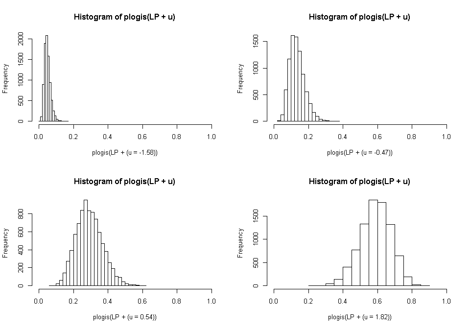
What you can see is that although the distribution is the same across all levels of the random effects (because we hold the random effects constant within a particular histogram), the position of the distribution varies tremendously. Thus simply ignoring the random effects and focusing on the fixed effects would paint a rather biased picture of the reality. Incorporating them, it seems that although there will definitely be within doctor variability due to the fixed effects (patient characteristics), there is more variability due to the doctor. Not incorporating random effects, we might conclude that in order to maximize remission, we should focus on diagnosing and treating people earlier (younger age), good relationships (marital status), and low levels of circulating pro-inflammatory cytokines (IL6). Including the random effects, we might conclude that we should focus on training doctors.

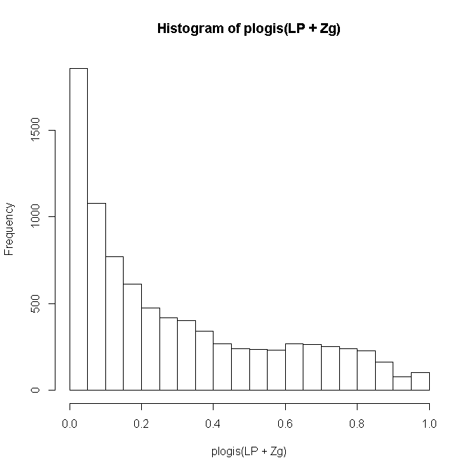
Finally, let’s look incorporate fixed and random effects for each individual and look at the distribution of predicted probabilities of remission in our sample. that is, now both fixed and random effects can vary for every person.

Count Outcomes

We could fit a similar model for a count outcome, number of tumors. Counts are often modeled as coming from a poisson distribution, with the canonical link being the log. We will do that here and use the same predictors as in the mixed effects logistic, predicting count from from Age, Married (yes = 1, no = 0), and IL6 (continuous). We allow the intercept to vary randomly by each doctor. We might make a summary table like this for the results.

Mixed Effects Poisson for Tumor Count

Parameter	Est.	SE	p-value	Exp(Est.)
Intercept	-.233	.057	<.001	.792
Age	.026	.001	<.001	1.026
Married (yes v no)	-.13	.013	<.001	.878
IL6	.005	.002	.025	1.005
${\mathrm{\Sigma }}_{intercept}^2$	.169
Npatients = 8,525		Ndoctors = 407

The interpretations again follow those for a regular poisson model, for a one unit increase in Age, the expected log count of tumors increases .026. People who are married are expected to have .13 lower log counts of tumors than people who are single. Finally, for a one unit increase in IL6, the expected log count of tumors increases .005.

It can be more useful to talk about expected counts rather than expected log counts. However, we get the same interpretational complication as with the logistic model. The expected counts are conditional on every other value being held constant again including the random doctor effects. So for example, we could say that people who are married are expected to have .878 times as many tumors as people who are not married, for people with the same doctor (or same random doctor effect) and holding age and IL6 constant.

Like we did with the mixed effects logistic model, we can plot histograms of the expected counts from our model for our entire sample, holding the random effects at specific values. Here at the 20th, 40th, 60th, and 80th percentiles. This gives us a sense of how much variability in tumor count can be expected by doctor (the position of the distribution) versus by fixed effects (the spread of the distribution within each graph).

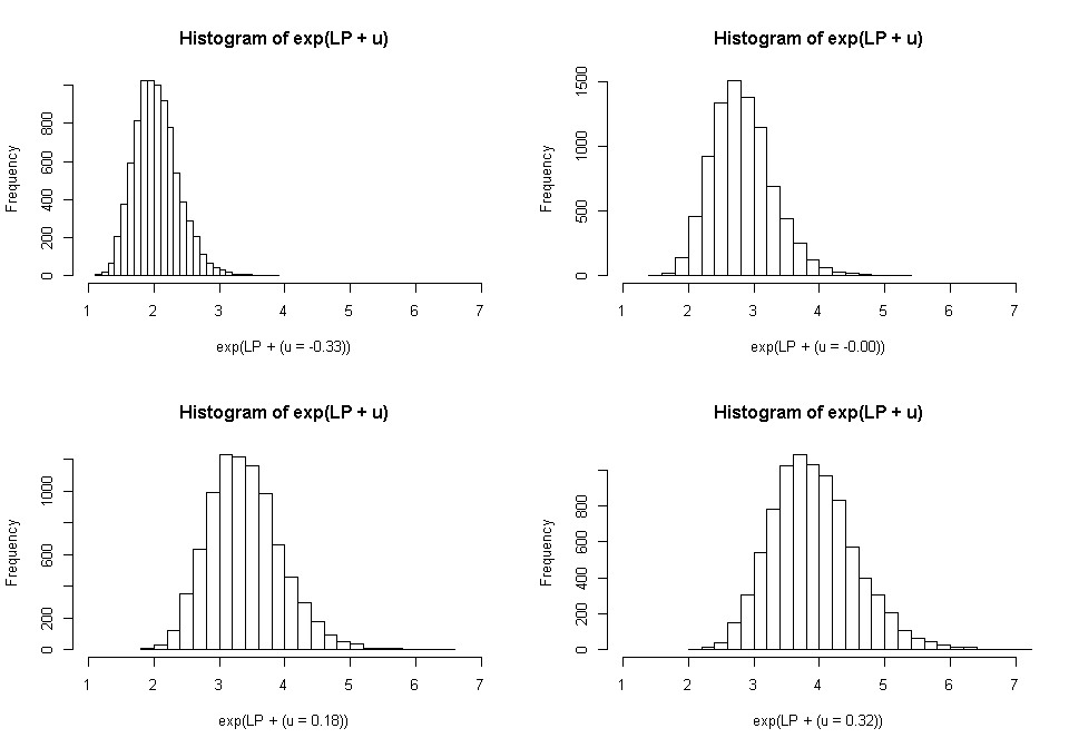
This time, there is less variability so the results are less dramatic than they were in the logistic example.

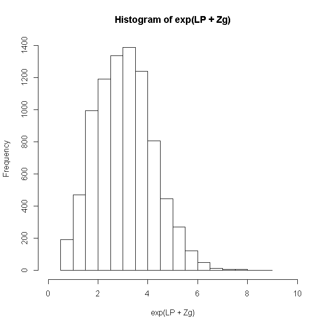
Finally, let’s look incorporate fixed and random effects for each individual and look at the distribution of expected tumor counts in our sample. that is, now both fixed and random effects can vary for every person.

Distribution Summary

	Normal (Gaussian)	Binomial	Poisson
Notation	$\mathcal{N}(\mu ,{\sigma }^2)$	$B(n,p)$	$Pois(\lambda )$
Parameters	$\mu \in \mathbb{R}$ & ${\mathrm{\Sigma }}^2\in \{\mathbb{R}\ge 0\}$	$n\in \{\mathbb{Z}\ge 0\}$ & $p\in [0,1]$	$\lambda \in \mathbb{R}\ge 0$
Support	$y\in \mathbb{R}$	$y\in \{0,\dots ,n\}$	$y\in \{\mathbb{Z}\ge 0\}$
Mean	$\mu$	$np$	$\lambda$
Variance	${\mathrm{\Sigma }}^2$	$np(1–p)$	$\lambda$
PDF/PMF	$\varphi (x)=\frac{1}{\sqrt{2\pi {\sigma }^2}}exp\{-\frac{(x–\mu {)}^2}{2{\sigma }^2}\}$	$\left(\begin{array}{c}n\\ k\end{array}\right)p^k(1–p{)}^{n–k}$	$\frac{{\lambda }^k}{k!}{e}^{-\lambda }$

Other Issues

For power and reliability of estimates, often the limiting factor is the sample size at the highest unit of analysis. For example, having 500 patients from each of ten doctors would give you a reasonable total number of observations, but not enough to get stable estimates of doctor effects nor of the doctor-to-doctor variation. 10 patients from each of 500 doctors (leading to the same total number of observations) would be preferable.

For parameter estimation, because there are not closed form solutions for GLMMs, you must use some approximation. Three are fairly common.

• Quasi-likelihood approaches use a Taylor series expansion to approximate the likelihood. Thus parameters are estimated to maximize the quasi-likelihood. that is, they are not true maximum likelihood estimates. A Taylor series uses a finite set of differentiations of a function to approximate the function, and power rule integration can be performed with Taylor series. With each additional term used, the approximation error decreases (at the limit, the Taylor series will equal the function), but the complexity of the Taylor polynomial also increases. Early quasi-likelihood methods tended to use a first order expansion, more recently a second order expansion is more common. In general, quasi-likelihood approaches are the fastest (although they can still be quite complex), which makes them useful for exploratory purposes and for large datasets. Because of the bias associated with them, quasi-likelihoods are not preferred for final models or statistical inference.
• The true likelihood can also be approximated using numerical integration. quadrature methods are common, and perhaps most common among these use the Gaussian quadrature rule, frequently with the Gauss-Hermite weighting function. It is also common to incorporate adaptive algorithms that adaptively vary the step size near points with high error. The accuracy increases as the number of integration points increases. Using a single integration point is equivalent to the so-called Laplace approximation. Each additional integration point will increase the number of computations and thus the speed to convergence, although it increases the accuracy. Adaptive Gauss-Hermite quadrature might sound very appealing and is in many ways. However, the number of function evaluations required grows exponentially as the number of dimensions increases. A random intercept is one dimension, adding a random slope would be two. For three level models with random intercepts and slopes, it is easy to create problems that are intractable with Gaussian quadrature. Consequently, it is a useful method when a high degree of accuracy is desired but performs poorly in high dimensional spaces, for large datasets, or if speed is a concern.
• A final set of methods particularly useful for multidimensional integrals are Monte Carlo methods including the famous Metropolis-Hastings algorithm and Gibbs sampling which are types of Markov chain Monte Carlo (MCMC) algorithms. Although Monte Carlo integration can be used in classical statistics, it is more common to see this approach used in Bayesian statistics.

Another issue that can occur during estimation is quasi or complete separation. Complete separation means that the outcome variable separate a predictor variable completely, leading perfect prediction by the predictor variable. Particularly if the outcome is skewed, there can also be problems with the random effects. For example, if one doctor only had a few patients and all of them either were in remission or were not, there will be no variability within that doctor.

References

• McCullagh, P, & Nelder, J. A. (1989). Generalized Linear Models, 2nd ed. Chapman & Hall/CRC Press.
• Agresti, A. (2013). Categorical Data Analysis, 3rd ed. John Wiley & Sons.
• Breslow, N. E. & Clayton, D. G. (1993). Approximate inference in generalized linear mixed models. Journal of the American Statistical Association, 88(421), pp 9-25, http://www.jstor.org/stable/2290687.
• Skrondal, A. & Rabe-Hesketh, S. (2004). Generalized Latent Variable Modeling: Multilevel, longitudinal, and structural equation models. Chapman & Hall/CRC Press.
• Pinheiro, J. C. & Chao, E. C. (2006). Efficient Laplacian and Adaptive Gaussian quadrature Algorithms for Multilevel Generalized Linear Mixed Models. Journal of Computational and Graphical Statistics, 15(1), pp 58-81, www.tandfonline.com/doi/abs/10.1198/106186006X96962.