The aim of this seminar is to help you learn about the use of Multilevel Modeling for the Analysis of Longitudinal Data. The seminar will feature examples from Applied Longitudinal Data Analysis: Modeling Change and Event Occurrence by Judith D. Singer and John B. Willett The seminar will address the following issues.
- A comparison of strategies for analyzing longitudinal data, including repeated measures ANOVA, mixed models analysis, regression, and multilevel modeling
- Multilevel models for analyzing longitudinal data
- Models for evaluating changes in “elevation” and “slope” over time.
- Using multilevel models to analyze “treatment effects” over time.
The seminar will focus on the construction and interpretation of these models with the aims of appealing to users of all multilevel modeling packages (e.g., HLM, SAS PROC MIXED, MLwiN, SPSS mixed, etc.). For the sake of realism, many examples will be run using HLM, but examples of using SAS PROC MIXED and MLwiN will also be included.
A comparison of strategies for analyzing longitudinal data
An Example : Kids’ alcohol use measured at 3 time points, age 14, 15, 16
- Everyone has the same number of waves of data (3 waves of data)
- All waves of data were measured at the same time (all measured on their birthday)
- Measures across time are probably not independent.
Strategies for Analyzing Longitudinal Data
- TraditionalRepeated Measures ANOVA
- It assumes that all kids have the same number of waves of data.
- It assumes all kids measured at the same time points (e.g. Sally cannot be measured at age 14,15.5, 16.5).
- Handles correlations among time points, assuming CS or UN.
-
proc glm data=alc ;
  model alcuse14 alcuse15 alcuse16 = coa / nouni ;
  repeated age 3 polynomial / summary;
run;
-
- Mixed Models Anova
- It is OK if some kids have more waves of data than others.
- The repeated statement assumes kids all measured at the same time points (for computing covariance structures).
- Handles correlations among time points, using mixed can even handle many
different kinds of covariance structures.
-
proc mixed data=alcpp ;
  class age;
  model alcuse = age coa age*coa / solution ;
  repeated age / subject=id type=ar(1) ;
run;
-
- Regression
- It is OK if some kids have more waves of data than others
- Do not need people measured on the same schedule
- Assumes no correlations among time points for a given person.
-
proc reg data=alcpp ;
  model alcuse = age coa ageBYcoa  ;
run;
-
- Multilevel Modeling
- It is OK if some kids have more waves of data
- It is OK if kids are measured on different schedules
- The covariance structure is based on the distance (in time) from each
other.
-
proc mixed data=alcpp ;
  class id;
  model alcuse = coa age coa*age / solution ;
  random intercept age / type=un sub=id;
run;
-
| Must have same number of waves of data | Must have same measurement schedule | Covariance Structures Permitted | Format of Data | |
| Traditional Repeated Measures | Yes | Yes | CS, UN | Person (Wide) |
| Mixed Repeated Measures | No | Yes (for covariance) | CS, UN, AR, and many others | Person Period (Long) |
| Regression | No | No | Independent | Person Period (Long) |
| Multilevel Model | No | No | A kind of AR, and others based on random effects. | Person Period (Long) |
Multilevel models for analyzing longitudinal data
- Applying the multilevel model to longitudinal data
- Studying alcohol use over time.
- Time is level 1, Person is level 2. Time is nested within persons.
- Just like students within classrooms
- We can ask about student level (level 1) characteristics the affect performance
- We can ask about “classroom” characteristics (level 2) that influence student performance.
- We can ask about “classroom” characteristics that influence the student level intercepts and slopes.
- In this example we can ask
- What time varying characteristics (level 1) affect alcohol use (e.g. time)
- What “person” characteristics (level 2) influence alcohol use (e.g. Peer drinking at start of study, being a child of an alcoholic).
- We can ask about “person” characteristics (level 2) that influence initial alcohol use (intercept) and change over time (slope).
Consider Figure 4.1, Page 1
Consider Table 4.2, Page 2
Consider Figure 4.1, Page 3
- We will examine Models A-E.
- We could use HLM, MLwiN, SAS Proc Mixed, SPSS Mixed, Splus, R, or Mplus to solve these
- Running the multilevel model is not hard, it is constructing and interpreting the model that is tricky. Once you have constructed the model, then putting it into the package is generally easy.
- We will show examples using HLM, but also show SAS Proc Mixed and MLwiN examples for final model.
Table 4.1, Model A
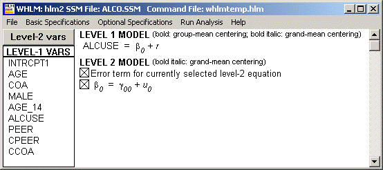
This is a simple “intercept only” model, predicting alcohol use from the overall mean.
Level 1/Level 2 model
ALCUSEij = π0i + εij π0i = γ00 + ζ0i
Composite model
ALCUSEij = γ00 + (εij + ζ0i )
Running model in HLM
 Final estimation of fixed effects:
 ----------------------------------------------------------------------------
                                       Standard             Approx.
    Fixed Effect         Coefficient   Error      T-ratio   d.f.     P-value
 ----------------------------------------------------------------------------
 For       INTRCPT1, B0
    INTRCPT2, G00           0.921955   0.095707     9.633        81    0.000
 ----------------------------------------------------------------------------
Final estimation of variance components: ----------------------------------------------------------------------------- Random Effect Standard Variance df Chi-square P-value Deviation Component ----------------------------------------------------------------------------- INTRCPT1, U0 0.75091 0.56386 81 328.92616 0.000 level-1, R 0.74950 0.56175 -----------------------------------------------------------------------------
Results as Level 1/Level 2 model
Fixed Effects
ALCUSEij = π0i + εij π0i = .92 + ζ0i
Variance Components
Level 1 Within Person, V(ε) = .563 Level 2 Initial Status, V(ζ0) = .561
Table 4.1, Model B
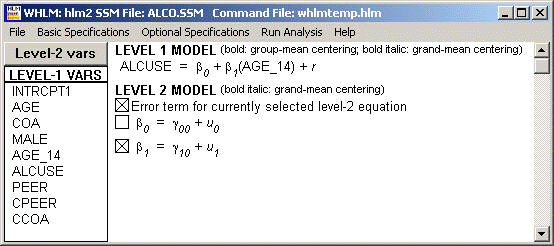
This model predicts alcohol use from the intercept and time, both of which randomly vary across children.
Level 1/Level 2 model
ALCUSEij = π0i + π1iTIME + εij π0i = γ00 + ζ0i π1i = γ10 + ζ1i
Composite model
ALCUSEij = γ00 + γ10 + (εij + ζ0i + ζ1iTIME )
Running Model in HLM
 Final estimation of fixed effects:
 ----------------------------------------------------------------------------
                                       Standard             Approx.
    Fixed Effect         Coefficient   Error      T-ratio   d.f.     P-value
 ----------------------------------------------------------------------------
 For       INTRCPT1, B0
    INTRCPT2, G00           0.651304   0.105080     6.198        81    0.000
 For   AGE_14 slope, B1
    INTRCPT2, G10           0.270651   0.062455     4.334        81    0.000
 ----------------------------------------------------------------------------
Final estimation of variance components: ----------------------------------------------------------------------------- Random Effect Standard Variance df Chi-square P-value Deviation Component ----------------------------------------------------------------------------- INTRCPT1, U0 0.79016 0.62436 81 264.14675 0.000 AGE_14 slope, U1 0.38885 0.15120 81 155.51848 0.000 level-1, R 0.58077 0.33729 -----------------------------------------------------------------------------
Results as Level 1/Level 2 model
Fixed Effects
ALCUSEij = π0i + π1iTIME + εij π0i = .65 + ζ0i π1i = .27 + ζ1i
Variance Components
Level 1 Within Person, V(ε) = .34 Level 2 Initial Status, V(ζ0) = .62 Rate of Change, V(ζ1) =.15 Cov(ζ0 , ζ1) = -.07
Table 4.1, Model C
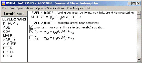
This model predicts alcohol use from the intercept and time. It also asks whether the intercept and slope (for time) are affected by being a child of an alcoholic.
Level 1/Level 2 model
ALCUSEij = π0i + π1iTIME + εij π0i = γ00 + γ01COA + ζ0i π1i = γ10 + γ11COA + ζ1i
Composite model
ALCUSEij = γ00 + γ01COA + γ10TIME + γ11COA*TIME + (εij + ζ0i + ζ1iTIME )
Running Model in HLM
 Final estimation of fixed effects:
 ----------------------------------------------------------------------------
                                       Standard             Approx.
    Fixed Effect         Coefficient   Error      T-ratio   d.f.     P-value
 ----------------------------------------------------------------------------
 For       INTRCPT1, B0
    INTRCPT2, G00           0.315952   0.130695     2.417        80    0.016
         COA, G01           0.743212   0.194566     3.820        80    0.000
 For   AGE_14 slope, B1
    INTRCPT2, G10           0.292955   0.084228     3.478        80    0.001
         COA, G11          -0.049430   0.125389    -0.394        80    0.693
 ----------------------------------------------------------------------------
Final estimation of variance components: ----------------------------------------------------------------------------- Random Effect Standard Variance df Chi-square P-value Deviation Component ----------------------------------------------------------------------------- INTRCPT1, U0 0.69827 0.48758 80 224.24420 0.000 AGE_14 slope, U1 0.38807 0.15060 80 155.22430 0.000 level-1, R 0.58077 0.33729 -----------------------------------------------------------------------------
Results as Level 1/Level 2 model
Fixed Effects
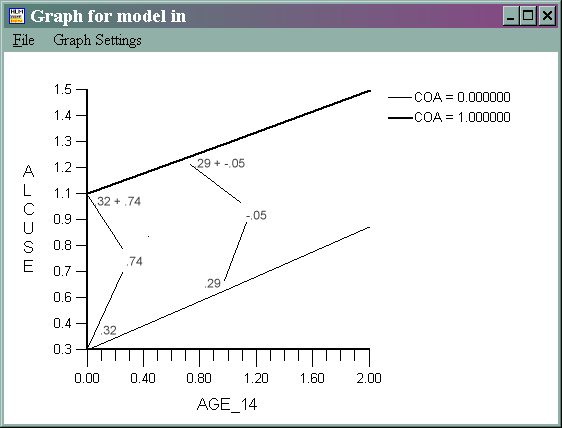
ALCUSEij = π0i + π1iTIME + εij π0i = .32 + .74COA + ζ0i π1i = .29 + -0.05COA + ζ1i
Variance Components
Level 1 Within Person, V(ε) = .34 Level 2 Initial Status, V(ζ0) = .48 Rate of Change, V(ζ1) =.15 Cov(ζ0 , ζ1) = -.06
We have graphed the results below, adding some annotations to help with interpretation.
Table 4.1, Model D
This model predicts alcohol use from the intercept and time. It also asks whether the intercept and slope (for time) are affected by being a child of an alcoholic and by amount of peer drinking (at the start of the study).
Level 1/Level 2 model
ALCUSEij = π0i + π1iTIME + εij π0i = γ00 + γ01COA + γ02PEER + ζ0i π1i = γ10 + γ11COA + γ12PEER + ζ1i
Composite model
ALCUSEij = γ00 + γ01COA + γ10TIME + γ10COA*TIME + γ02PEER + γ12PEER*TIME + (εij + ζ0i + ζ1iTIME )
Running Model in HLM
 Final estimation of fixed effects:
 ----------------------------------------------------------------------------
                                       Standard             Approx.
    Fixed Effect         Coefficient   Error      T-ratio   d.f.     P-value
 ----------------------------------------------------------------------------
 For       INTRCPT1, B0
    INTRCPT2, G00          -0.316514   0.148062    -2.138        79    0.032
         COA, G01           0.579165   0.162486     3.564        79    0.001
        PEER, G02           0.694296   0.111533     6.225        79    0.000
 For   AGE_14 slope, B1
    INTRCPT2, G10           0.429429   0.113689     3.777        79    0.000
         COA, G11          -0.014032   0.124765    -0.112        79    0.911
        PEER, G12          -0.149815   0.085641    -1.749        79    0.080
 ----------------------------------------------------------------------------
Final estimation of variance components: ----------------------------------------------------------------------------- Random Effect Standard Variance df Chi-square P-value Deviation Component ----------------------------------------------------------------------------- INTRCPT1, U0 0.49082 0.24091 79 152.28049 0.000 AGE_14 slope, U1 0.37298 0.13911 79 149.63981 0.000 level-1, R 0.58077 0.33729 -----------------------------------------------------------------------------Statistics for current covariance components model -------------------------------------------------- Deviance = 588.690655 Number of estimated parameters = 10
Results as Level 1/Level 2 model
Fixed Effects
ALCUSEij = π0i + π1iTIME + εij π0i = -.31 + .57COA + .69PEER + ζ0i π1i = .43 + -.01COA+ -.15PEER + ζ1i
Variance Components
Level 1 Within Person, V(ε) = .34 Level 2 Initial Status, V(ζ0) = .24 Rate of Change, V(ζ1) =.14 Cov(ζ0 , ζ1) = -.006
Table 4.1, Model E
This model is the same as model D, but removes COA as a predictor of the slope for age_14.
Level 1/Level 2 model
ALCUSEij = π0i + π1iTIME + εij π0i = γ00 + γ01COA + γ02PEER + ζ0i π1i = γ10 + γ12PEER + ζ1i
Composite model
ALCUSEij = γ00 + γ01COA + γ10TIME + γ02PEER + γ12PEER*TIME + (εij + ζ0i + ζ1iTIME )
Running Model using HLM
 Final estimation of fixed effects:
 ----------------------------------------------------------------------------
                                       Standard             Approx.
    Fixed Effect         Coefficient   Error      T-ratio   d.f.     P-value
 ----------------------------------------------------------------------------
 For       INTRCPT1, B0
    INTRCPT2, G00          -0.313821   0.146118    -2.148        79    0.032
         COA, G01           0.571196   0.146228     3.906        79    0.000
        PEER, G02           0.695183   0.111258     6.248        79    0.000
 For   AGE_14 slope, B1
    INTRCPT2, G10           0.424687   0.105590     4.022        80    0.000
        PEER, G11          -0.151377   0.084513    -1.791        80    0.073
 ----------------------------------------------------------------------------
Final estimation of variance components: ----------------------------------------------------------------------------- Random Effect Standard Variance df Chi-square P-value Deviation Component ----------------------------------------------------------------------------- INTRCPT1, U0 0.49086 0.24095 79 152.28729 0.000 AGE_14 slope, U1 0.37305 0.13916 80 149.66517 0.000 level-1, R 0.58076 0.33729 -----------------------------------------------------------------------------
Results as Level 1/Level 2 model
Fixed Effects
ALCUSEij = π0i + π1iTIME + εij π0i = -.31 + .57COA + .70PEER + ζ0i π1i = .42 + -.15PEER + ζ1i
Variance Components
Level 1 Within Person, V(ε) = .34 Level 2 Initial Status, V(ζ0) = .24 Rate of Change, V(ζ1) =.14 Cov(ζ0 , ζ1) = -.006
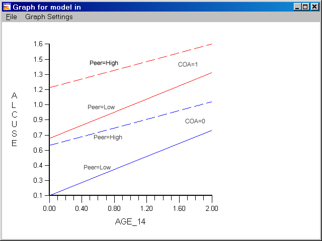
Graphing
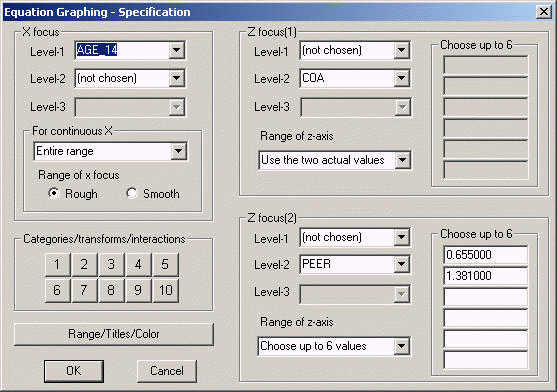
We treat a value for Peer of .65 as being low peer drinking and Peer of 1.38 as high peer drinking in the graph below. For ease of interpretation, graph was touched up in a graph editing program.
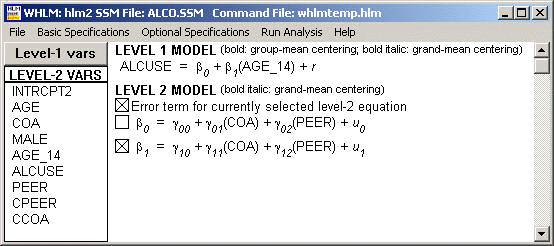
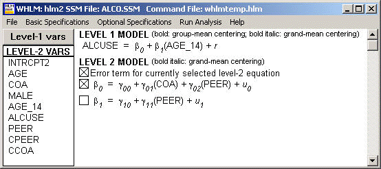
Here is how we made the graph in HLM.
Running Model E using SAS
Level 1/Level 2 model
ALCUSEij = π0i + π1iTIME + εij π0i = γ00 + γ01COA + γ02PEER + ζ0i π1i = γ10 + γ12PEER + ζ1i
Composite model
ALCUSEij = γ00 + γ01COA + γ10TIME + γ02PEER + γ12PEER*TIME + (εij + ζ0i + ζ1iTIME )
We then convert the composite model into a model statement with the fixed effects and random statement with the random effects.
proc mixed data="c:aldaalcohol1_pp" method=ml covtest;
  class id;
  model alcuse = coa age_14 peer peer*age_14 / solution ;
  random intercept age_14 / type=un sub=id;
run;
And here is the output
                  Covariance Parameter Estimates
                                    Standard         Z
Cov Parm     Subject    Estimate       Error     Value        Pr Z
UN(1,1)      ID           0.2409     0.09259      2.60      0.0046
UN(2,1)      ID         -0.00614     0.05501     -0.11      0.9111
UN(2,2)      ID           0.1392     0.05481      2.54      0.0056
Residual                  0.3373     0.05268      6.40      <.0001

                    Solution for Fixed Effects
                           Standard
Effect         Estimate       Error      DF    t Value    Pr > |t|
Intercept       -0.3138      0.1461      79      -2.15      0.0348
COA              0.5712      0.1462      82       3.91      0.0002
PEER             0.6952      0.1113      82       6.25      <.0001
AGE_14           0.4247      0.1056      80       4.02      0.0001
PEER*AGE_14     -0.1514     0.08451      82      -1.79      0.0770
Composite model
ALCUSEij = γ00 + γ01COA + γ10TIME + γ02PEER + γ12PEER*TIME + (εij + ζ0i + ζ1iTIME )
with values of parameter estimates filled in.
ALCUSEij = -.31+ .57COA + .42TIME + .69PEER + -.15PEER*TIME + (εij + ζ0i + ζ1iTIME )
Results as Level 1/Level 2 model
ALCUSEij = π0i + π1iTIME + εij π0i = γ00 + γ01COA + γ02PEER + ζ0i π1i = γ10 + γ12PEER + ζ1i
With values of parameter estimates filled in.
ALCUSEij = π0i + π1iTIME + εij π0i = -.31 + .57COA + .69PEER + ζ0i π1i = .42 + -.15PEER + ζ1i
Running Model E using MLwiN
Level 1/Level 2 model
ALCUSEij = π0i + π1iTIME + εij π0i = γ00 + γ01COA + γ02PEER + ζ0i π1i = γ10 + γ12PEER + ζ1i
Composite model
ALCUSEij = γ00 + γ01COA + γ10TIME + γ02PEER + γ12PEER*TIME + (εij + ζ0i + ζ1iTIME )
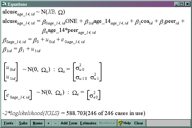
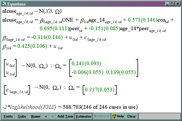
We then form the MLwiN model with all of the fixed effects listed above. A random effects at level 1 is specified for the intercept to specify εij and a random effect for the intercept at level 2 is specified to create ζ0i . A random effect for age_14 is specified to create ζ1iTIME.
and the results are
Using multilevel models to analyze “treatment effects” over time.
- Studying effect of “antidepressant” on mood over 7 days, 3 measurements per day (21 total measures).
- We could number time 0, 1, 2… 20 but then lose the meaning of day.
- If we divide by 3, then a “one unit increase” corresponds to a one day increase in time, so time goes 0, .33, .67, 1 … 6, 6.33, 6.67
- Patients randomly assigned to “placebo” or “treatment” groups.
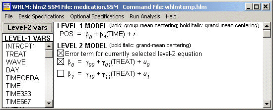
Table 5.10, Model A: TIME centered at 0 (start of study)
Level 1/Level 2 model
POSij = π0i + π1iTIME + εij π0i = γ00 + γ01TREAT + ζ0i π1i = γ10 + γ11TREAT + ζ1i
Composite model
POSij = γ00 + γ01TREAT + γ10TIME + γ11TREAT*TIME + (εij + ζ0i + ζ1iTIME )
 Final estimation of fixed effects:
 ----------------------------------------------------------------------------
                                       Standard             Approx.
    Fixed Effect         Coefficient   Error      T-ratio   d.f.     P-value
 ----------------------------------------------------------------------------
 For       INTRCPT1, B0
    INTRCPT2, G00         167.463464   9.326039    17.957        62    0.000
       TREAT, G01          -3.109319  12.332266    -0.252        62    0.801
 For     TIME slope, B1
    INTRCPT2, G10          -2.418121   1.730814    -1.397        62    0.162
       TREAT, G11           5.536805   2.277796     2.431        62    0.015
 ----------------------------------------------------------------------------
Final estimation of variance components: ----------------------------------------------------------------------------- Random Effect Standard Variance df Chi-square P-value Deviation Component ----------------------------------------------------------------------------- INTRCPT1, U0 45.94957 2111.36260 62 629.96490 0.000 TIME slope, U1 7.98338 63.73439 62 315.00708 0.000 level-1, R 35.07037 1229.93068 -----------------------------------------------------------------------------Treatment effect is difference between groups at start of study, see page 4, Figure 5.5
Model B: TIME-3.33 (middle of study)
See Page 5, Table 5.9
Level 1/Level 2 model
POSij = π0i + π1i(TIME-3.33) + εij π0i = γ00 + γ01TREAT + ζ0i π1i = γ10 + γ11TREAT + ζ1i
Composite model
POSij = γ00 + γ01TREAT + γ10(TIME-3.33) + γ11TREAT*(TIME-3.33) + (εij + ζ0i + ζ1i(TIME-3.33) )
 Final estimation of fixed effects:
 ----------------------------------------------------------------------------
                                       Standard             Approx.
    Fixed Effect         Coefficient   Error      T-ratio   d.f.     P-value
 ----------------------------------------------------------------------------
 For       INTRCPT1, B0
    INTRCPT2, G00         159.403064   8.764424    18.188        62    0.000
       TREAT, G01          15.346694  11.544537     1.329        62    0.184
 For  TIME333 slope, B1
    INTRCPT2, G10          -2.418118   1.730816    -1.397        62    0.162
       TREAT, G11           5.536811   2.277798     2.431        62    0.015
 ----------------------------------------------------------------------------
Final estimation of variance components: ----------------------------------------------------------------------------- Random Effect Standard Variance df Chi-square P-value Deviation Component ----------------------------------------------------------------------------- INTRCPT1, U0 44.81918 2008.75915 62 2052.73713 0.000 TIME333 slope, U1 7.98338 63.73439 62 315.00698 0.000 level-1, R 35.07037 1229.93106 -----------------------------------------------------------------------------Treatment effect is difference between groups half-way through study, see page 4, Figure 5.5
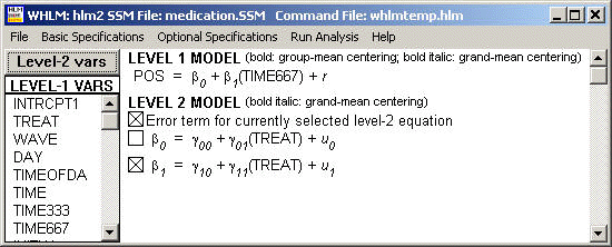
Model C: TIME-6.67 (end of study)
See Page 5, Table 5.9
Level 1/Level 2 model
POSij = π0i + π1i(TIME-6.67) + εij π0i = γ00 + γ01TREAT + ζ0i π1i = γ10 + γ11TREAT + ζ1i
Composite model
POSij = γ00 + γ01TREAT + γ10(TIME-6.67) + γ11TREAT*(TIME-6.67) + (εij + ζ0i + ζ1i(TIME-6.67) )
 Final estimation of fixed effects:
 ----------------------------------------------------------------------------
                                       Standard             Approx.
    Fixed Effect         Coefficient   Error      T-ratio   d.f.     P-value
 ----------------------------------------------------------------------------
 For       INTRCPT1, B0
    INTRCPT2, G00         151.342994  11.542088    13.112        62    0.000
       TREAT, G01          33.802434  15.157594     2.230        62    0.026
 For  TIME667 slope, B1
    INTRCPT2, G10          -2.418048   1.730569    -1.397        62    0.162
       TREAT, G11           5.536745   2.277472     2.431        62    0.015
 ----------------------------------------------------------------------------
Final estimation of variance components: ----------------------------------------------------------------------------- Random Effect Standard Variance df Chi-square P-value Deviation Component ----------------------------------------------------------------------------- INTRCPT1, U0 57.64097 3322.48125 62 931.61025 0.000 TIME667 slope, U1 7.98347 63.73582 62 315.00715 0.000 level-1, R 35.07036 1229.92993 -----------------------------------------------------------------------------Treatment effect is difference between groups at end of study, see page 4, Figure 5.5
See summary of results on Page 6, 5.10
Models for evaluating changes in “elevation” and “slope” over time.
See Figure 6.1, page 7 for different kinds of change in elevation and slope.
We will consider the following 4 models
See Figure 6.2, page 8 for the 4 models we will test.
-
Figure 6.2a: Change in elevation
-
Figure 6.2b: Change in slope
-
Figure 6.2c: Change in elevation and slope
-
Figure 6.2d: Change in elevation and slope (method 2)
Change in elevation, Figure 6.2a, Page 8
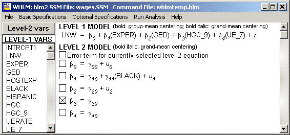
Level 1 Model (focusing on “exper” and “ged”, ignoring covariates)
LNWij = π0i + π1iEXPER + π2iGED + εij
Running Model in HLM
 Final estimation of fixed effects:
 ----------------------------------------------------------------------------
                                       Standard             Approx.
    Fixed Effect         Coefficient   Error      T-ratio   d.f.     P-value
 ----------------------------------------------------------------------------
 For       INTRCPT1, B0
    INTRCPT2, G00           1.734212   0.011800   146.971       887    0.000
 For    EXPER slope, B1
    INTRCPT2, G10           0.043224   0.002621    16.490       886    0.000
       BLACK, G11          -0.018200   0.004471    -4.071       886    0.000
 For      GED slope, B2
    INTRCPT2, G20           0.061321   0.018449     3.324       887    0.001
 For    HGC_9 slope, B3
    INTRCPT2, G30           0.038334   0.006265     6.119      6396    0.000
 For     UE_7 slope, B4
    INTRCPT2, G40          -0.011609   0.001788    -6.494      6396    0.000
 ----------------------------------------------------------------------------
Final estimation of variance components: ----------------------------------------------------------------------------- Random Effect Standard Variance df Chi-square P-value Deviation Component ----------------------------------------------------------------------------- INTRCPT1, U0 0.20882 0.04361 103 146.13199 0.004 EXPER slope, U1 0.04075 0.00166 102 177.35923 0.000 GED slope, U2 0.16823 0.02830 103 109.96355 0.301 level-1, R 0.30686 0.09416 -----------------------------------------------------------------------------
Model D: Change in slope, Figure 6.2b, Page 8
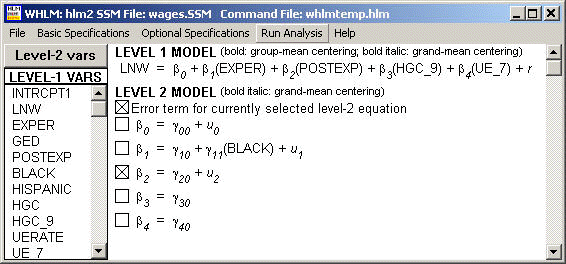
In addition to exper (time in work force) also have postexp (time in work force after getting GED).
See page 9, Table 6.1 for data example.
Level 1 Model (focusing on “exper” and “postexp”)
LNWij = π0i + π1iEXPER + π3iPOSTEXP + εij
Running Model in HLM
 Final estimation of fixed effects:
 ----------------------------------------------------------------------------
                                       Standard             Approx.
    Fixed Effect         Coefficient   Error      T-ratio   d.f.     P-value
 ----------------------------------------------------------------------------
 For       INTRCPT1, B0
    INTRCPT2, G00           1.749372   0.011399   153.461       887    0.000
 For    EXPER slope, B1
    INTRCPT2, G10           0.040653   0.002777    14.637       886    0.000
       BLACK, G11          -0.019495   0.004475    -4.357       886    0.000
 For  POSTEXP slope, B2
    INTRCPT2, G20           0.014591   0.004565     3.196       887    0.002
 For    HGC_9 slope, B3
    INTRCPT2, G30           0.039868   0.006354     6.275      6396    0.000
 For     UE_7 slope, B4
    INTRCPT2, G40          -0.011839   0.001791    -6.612      6396    0.000
 ----------------------------------------------------------------------------
Final estimation of variance components: ----------------------------------------------------------------------------- Random Effect Standard Variance df Chi-square P-value Deviation Component ----------------------------------------------------------------------------- INTRCPT1, U0 0.22488 0.05057 95 97.32352 0.415 EXPER slope, U1 0.03805 0.00145 94 128.15709 0.011 POSTEXP slope, U2 0.02891 0.00084 95 124.13282 0.024 level-1, R 0.30764 0.09464 -----------------------------------------------------------------------------
Model F: Change in elevation and slope, Figure 6.2c, Page 8
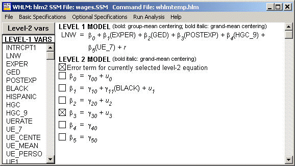
Level 1 Model (focusing on “exper” and “postexp”)
LNWij = π0i + π1iEXPER + π2iGED + π3iPOSTEXP + εij
Running Model in HLM
 Final estimation of fixed effects:
 ----------------------------------------------------------------------------
                                       Standard             Approx.
    Fixed Effect         Coefficient   Error      T-ratio   d.f.     P-value
 ----------------------------------------------------------------------------
 For       INTRCPT1, B0
    INTRCPT2, G00           1.738550   0.011949   145.498       887    0.000
 For    EXPER slope, B1
    INTRCPT2, G10           0.041475   0.002798    14.824       886    0.000
       BLACK, G11          -0.019620   0.004470    -4.389       886    0.000
 For      GED slope, B2
    INTRCPT2, G20           0.040940   0.022022     1.859       887    0.063
 For  POSTEXP slope, B3
    INTRCPT2, G30           0.009412   0.005546     1.697       887    0.089
 For    HGC_9 slope, B4
    INTRCPT2, G40           0.039032   0.006243     6.252      6395    0.000
 For     UE_7 slope, B5
    INTRCPT2, G50          -0.011723   0.001783    -6.575      6395    0.000
 ----------------------------------------------------------------------------
Final estimation of variance components: ----------------------------------------------------------------------------- Random Effect Standard Variance df Chi-square P-value Deviation Component ----------------------------------------------------------------------------- INTRCPT1, U0 0.20336 0.04135 60 79.33686 0.048 EXPER slope, U1 0.03690 0.00136 59 70.25123 0.150 GED slope, U2 0.13172 0.01735 60 45.99434 >.500 POSTEXP slope, U3 0.05801 0.00336 60 66.49441 0.263 level-1, R 0.30637 0.09386 -----------------------------------------------------------------------------
Figure 6.2d: Change in elevation and slope (method 2)
- See page 9, Table 6.1. If we include ged*exper to reflect change in slope after ged, then what is the meaning of ged effect? The effect of getting ged on the day you enter the labor force.
Summary
Multilevel modeling offers a unique framework for analyzing longitudinal data because
- It tolerates missing waves of data
- It tolerates differently spaced waves of data from different subjects
- It accounts for correlations of observations across time
- It allows you to study changes over time, such as changes in elevation and slope.
- You are not limited just to linear changes, but can explore a variety of functional forms of change over time.
For more information
- Applied Longitudinal Data Analysis: Modeling Change and Event Occurrence by Judith D. Singer and John B. Willett

