This example is taken from Levy and Lemeshow’s Sampling of Populations.
page 109 repeated systematic sampling
A short "movie" of how to convert the SAS data set wvwloss2 into a WesVar data set can be viewed by clicking here. A new variable called cons was added to the wloss data set. This variable is a constant that is equal to one for all cases. This variable was added for use in making the table. Because cons had only one value, it adds only one row to the table, making the table easier to read.
A second "movie" shows how to analyze the data once it is in WesVar format. You can view that movie by clicking here.
In this example, the variable wt1 is used as the weight variable, the variable cluster is used as the VarUnit and the variable xi is used as the analysis variable. The jackknife1 (jk1) method of creating the replicate weight is used because we do not have stratification in this design.
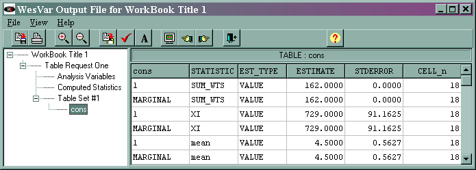
The output (shown at the end of the analysis "movie") is given below.
The marginal sum_wts value of 162 is the estimated population total. The marginal xi value of 729 is the estimated total of the variable xi, and its standard error is 91.1625. The marginal mean value of 4.5 is the estimated mean of the variable xi, and 0.5627 is its standard error. The standard error for the total and the mean are different from those produced by SUDAAN because of the different way in which the two packages calculate the FPCs. If an FPC of .703 is used in WesVar, results very similar to SUDAAN’s will be obtained.

