This example is taken from Levy and Lemeshow’s Sampling of Populations.
page 53 simple random sampling
Below are some brief notes regarding the importing of data into WesVar below. Despite the length of the material below, the process is short and simple. The written material looks extensive only because it takes many words to describe relatively few point-and-click actions.
Note that a new variable, called psu, was added to the data set while it was still in SAS. This variable is just a counting variable (i.e., an index or an identification variable) that will be used as the PSU (primary sampling unit) variable.
When using a simple random sampling design, the only elements that you will need to identify to WesVar are the weight variable, the PSU variable, which WesVar calls the VarUnit, and the analysis variable. In this example, the weight variable is called weight1, the VarUnit is called psu, and the analysis variable is called momsag. We will use the jackknife1 (jk1) method because we do not have stratification in our sample design.
Overview of importing data into WesVar
Many people are familiar with converting their data from one format to another, say from SAS to SPSS format, by using a non-statistical program such as Stat/Transfer or DBMS/Copy. WesVar is one of the few statistical packages for which this method of format conversion will not work (because these programs cannot tell WesVar how the replicate weights were created). You can import into WesVar data sets that contain either PSU and (possibly) strata variables, or you can import data files that already contain the replicate weight variables. Most of our examples show how to import data files that contain PSU and strata variables and show how to create the replicate weights within WesVar. However, we will note what to do if your data set already contains the replicate weight variables. In either case, once you open WesVar, you will be presented with a screen with four options: create a new WesVar data file, open a data file that is already in WesVar format, create a new workbook or open an existing workbook. We will click on the red button in the upper left of the screen to create a new WesVar data file. After selecting the data file to be imported, you will need to indicate to WesVar some key variables. To do this, click on the radio button next to the type of variable and then select and move the variable into the box. The only two variables that you must identify is the full sample weight variable (usually the p-weight) and the variables. All of the variables in the variables box can be used as variables in any analysis. You can use the double arrow to move all of the variables at once. If you indicate a variable as in ID variable, that variable will not be available for any other use, such as a PSU variable. There will be no problem if you have an ID variable in your data set and you do not indicate it as such. If you have replicate weights in your data set, you would put those variables in the replicates box. Note that you can use the buttons with the double arrows to move all of the variables in the direction of the arrows by clicking on that button. Next, you will need to save the data file before you can proceed. Click on “file” and “save as” to do this. You will find information about what you need to do next in the lower left-hand corner of the window. Also, an explanation of each of the boxes will appear if you leave your cursor on the box for a few moments.
Now that you have saved your file, it is time to create the replicate weights. Click on “data” at the top of the menu bar and select “create weights”. Choose the type of replicate weight by clicking on the appropriate radio button on the right. The type of replicate weight that should be used depends on the design of your survey. For a simple random sample design, we will use jackknife 1 (jk1) because we do not have stratification. Click on the radio button to indicate the “VarUnit” variable. In this box you will indicate the PSU variable. If we had a stratified sample, we would click on the “VarStrat” radio button and put the strata variable in that box. Now we will click on OK and save the data file. WesVar will ask if you want to replace the existing data file. In our examples, we always say yes. However, if you are uncertain about which type of replicate weights to create, you can rename the current data file. By doing this, you will have two WesVar data files: one that does not have replicate weights (which you will not be able to analyze until you create replicate weights) and one with the replicate weights. You are now ready to analyze your data in WesVar.
Overview of analyzing the data in WesVar
We begin by opening a new WesVar workbook. All analyses are done inside of a workbook. To begin, click on “New WesVar Workbook” from the main page. Once the data set has been selected, you have the option of creating a table (i.e., doing descriptive statistics) or conducting regression analyses. After selecting to create a table, you are asked if you want to create a single or multiple table set. In this example, we will create a single table. After making this selection, you will notice that the WesVar screen will be divided down the middle. Note that the options available to you on the right side of the screen will change as you select different nodes on the tree on the left of the screen. By clicking on “Table Set 1” on the right you can select the variable(s) you want used in the table. Don’t forget to click on “Add New Entry” to avoid getting an error message. Although you do not have to select an analysis variable, we do for the sake of clarity. The analysis variable can be different from the variable(s) used to create the table. Remember that at any time you see the double arrow, you can use it to move all of the variables in the direction of the arrows by clicking on the button. When computing statistics, you need to provide an equation in the form of new_variable_name = function(variable), where the function is something that you select from the pull-down menu or a formula that you provide. If you hold your cursor over the computed statistics box for a few seconds, an example will appear to the lower right of your cursor. Although we show how to get the mean of a variable by using the pull-down menu, you could also obtain the mean by clicking on the variable and then clicking on the “block mean” button. Note that WesVar will name the mean for you by adding M_ to the beginning of the variable name. If you need to include an FPC or want to change the alpha level, click on the options node of the tree. Please note that you can perform any of the tasks listed above in any order: unlike importing data, there is no specific order in which you must do these things. Also note that you can change the WorkBook Title 1 and Table Request One to anything that you like by clicking on these and supplying the new name in the dialogue box on the right. Changing these defaults is useful if you will be creating multiple workbooks or creating numerous tables within a single workbook. When you care ready, click on the green arrow (triangle) at the top to run your analysis. No output will appear. To see the output, click on Requests (at the top of the widow in the menu bar) and then View Output. The output window is set up in much the same way as the workbook window with a divided window with a tree on the left. As you expand the tree, you will see the various elements of the output. To view an element, click on it. As with the workbook window, the information displayed on the right will change depending on the item you click on the left. To return to the analysis window, you will need to close the output window. You can do this by clicking on the “X” at the top right of the window. Although it may seem like you are closing the WesVar program, you are only closing one window; the program will remain open for you to perform other analyses, etc.
The output (shown at the end of the analysis “movie”) is given below.
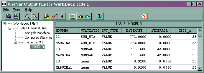
For most situations, only the values given on the lines that say “MARGINAL” are of interest. The other values listed in the column, called “HOSPNO” in this example, are the values of that variable. In this example, there is only one value of hospno and that is 13. If we had selected a different variable as the analysis variable, the values and the name of the column would reflect that variable. The marginal sum_wts value of 773 is the estimated population total. The marginal momsag value of 711.16 is the estimated total for the variable momsag, and its standard error is 42.8068. The marginal mean value of 0.92 is the estimated mean of the variable momsag, and its standard error is 0.0554. The column labeled CELL_n gives the number of observations in each cell.
This example is taken from Lehtonen and Pahkinen’s Practical Methods for Design and Analysis of Complex Surveys.
page 29 Table 2.4 Estimates from a simple random sample drawn without replacement (n = 8); the Province’91 population. The SAS data set page29 is used.
In this example, the variable wt is used as the weight variable, cluster is used as the VarUnit, and ue91 is used as the analysis variable. Because the sampling design was a simple random sample, we use the jackknife1 (jk1) method of creating the replicate weights. Also note that because the sample size is large relative to the population (eight elements sampled from a population of 32 elements), we need to use a finite population correction (FPC). To calculate the FPC, use the formula 1 – (n/N), where n is the sample size and N is the size of the population. In this case, 1 – (8/32) = .75. The value .75 is entered in the box called FPC which is shown when you click on the options node in the analysis window. Note that most other statistical packages do not ask you to calculate the FPC, but rather they calculate it for you based on other information that you provide.
The output is given below.
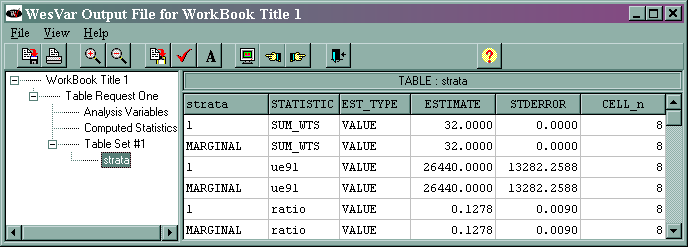
The marginal sum_wts value of 32 is the estimated population total. The marginal ue91 value of 26440 is the estimated total of the variable ue91, and its standard error is 13282.2588. The marginal ratio value of 0.1278 is the estimated ratio of ue91/lab91, and its standard error is 0.0090. This is slightly different from what is shown in the text, and we do not know why. The output for the median is not shown above. The median and its standard error are different from those shown in the text. We suspect that this might reflect a difference in the algorithms used by the different statistical packages.
Calculating ratios with a simple random sample
This example is taken from Levy and Lemeshow’s Sampling of Populations.
page 200 ratio estimation
The SAS data set tab7pt1 is used in the example.
In this example, the variable wt1 is used as the weight variable, the variable area is used as the VarUnit, and the variable totmedex is used as the analysis variable. The variable totcnt is used to make the table. The variable totcnt was selected as the variable used to make the table because it only has one value; hence, it only adds one row to the table entries, making the table easier to read. The jackknife-1 (jk1) method of creating the replicate weight is used because we do not have stratification in this design.
The output is given below.
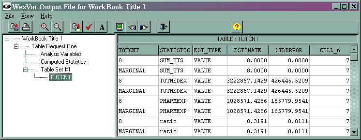
The marginal sum_wts value of 8 is the estimated population total. The marginal totmedex value of 3222857.1429 is the estimated total of the variable totmedex, and its standard error is 150771.2598. The marginal phramexp value of 1028571.4286 is the estimated total of pharmexp, and its standard error is 58612.0649. The marginal ratio value of 0.3191 is the estimated ratio of pharmexp/totmedex, and its standard error is 0.0039.


