This example is taken from Lehtonen and Pahkinen’s Practical Methods for Design and Analysis of Complex Surveys.
page 46 Table 2.6 Estimates from a systematic sample drawn from the Province’91 population using implicit stratification.
The SAS data file for this example can be downloaded by clicking here. Note that a modification was made to this data set: variables called cons and psu were added to the data set. The variable cons was added for use in making the table. The variable cons is equal to one for all cases. The variable psu was added for use as the VarUnit variable. While other survey data analysis packages, such as Stata, SAS and SUDAAN have the variable clu specified as the PSU variable, WesVar requires that the variable specified as the VarUnit be numbered starting from one within each strata. Hence, we needed to create this variable. We did this while the data were still in SAS using the code below.
data wvpage74;
  set page74;
  psu = _n_;
  if strata = 2 then psu = psu - 2;
  cons = 1;
run;
In this example, the variable wt is used as the weight variable, the variable psu is used as the VarUnit and the variable str is used as the StratVar (the variable that defines the strata). The jackknife-n (jkn) method of creating the replicate weights is used because it allows more than two PSUs per strata (as we have in strata 2). Also, we will need to use an FPC of .75 (1 – (8/32) = .75).
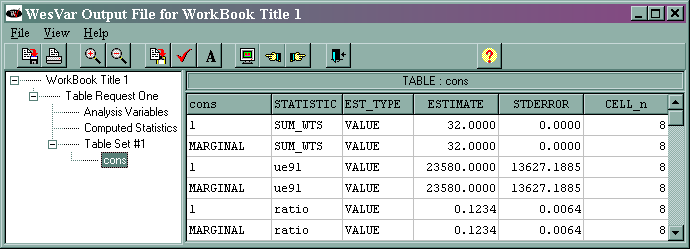
The output (shown at the end of the analysis “movie”) is given below.
The marginal sum_wts value of 32 is the estimated population total. The marginal ue91 value of 23580 is the estimated total of the variable ue91, and its standard error is 13627.1885 (this value is different from the value given in the text, and we do not know why). The marginal ratio value of 0.1234 is the estimated ratio of ue91/lab91, and its standard error is 0.0064.

