This example is taken from Levy and Lemeshow’s Sampling of Populations.
page 138 stratified random sampling
The SAS data set wvhospsamp is used in the example. Please note that some modifications were made to the hospsamp data set provided by Levy and Lemeshow to facilitate the analysis in WesVar. While the data were still in SAS, a variable called psu was added. This variable was created using the following SAS code:
data wvhospsamp;
  set hospsamp;
  psu = _n_;
  if oblevel = 2 then psu = psu - 4;
  if oblevel = 3 then psu = psu - 9;
run;
The point of this code is to create a new variable, that we called psu, that counts each observation within each level of the variable oblevel. This is necessary for analysis in WesVar. If psu was not consecutive numbers starting from 1 within each level of oblevel, WesVar would give an error message and the analysis could not be completed. Because the sampling rate is different within the levels of oblevel, we must use the “Attach Factors” feature of WesVar to give the appropriate FPCs for each level of oblevel. To calculate each FPC, use the formula 1 – (n/N), where n is the size of the sample and N is the size of the population. Hence, the calculation for level 1 of oblevel would be 1 – (4/42) = .9047619; for level 2, 1 – (5/99) = .949495, for level 3, 1 – (6/17) = .64705882. While calculations to this many decimal places is not required, rounding to two or three decimal places will slightly alter the results. Also note that, in the “movie”, when WesVar asks about saving the FPCs to an external data file, we decline. In many situations it may be a good idea to save the FPCs for future use or reference.
In this example, the variable weighta is used as the weight variable, the variable psu is used as the VarUnit, the variable oblevel is used as the VarStrat and the variable births is used as the analysis variable. The jackknife-n (jkn) method of creating the replicate weight is used because we do not always have exactly two PSUs per stratum in this design. The table is created using oblevel by births to give all of the information shown in the text (but it is still a “single” table).
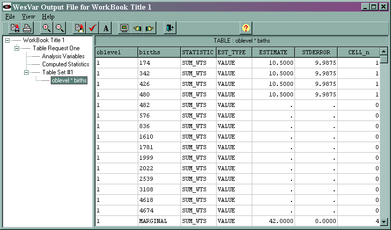
Part of the output is given below. Because the output is extensive, only part of it is shown as it appears in WesVar. For the rest of the output, the export function was used to export the output to a text file. This text file was edited to show only the relevant values.
 NUMBER OF REPLICATES :	15
 NUMBER OF OBSERVATIONS READ :	15
 WEIGHTED NUMBER OF OBSERVATIONS READ :	158.000


TABLE : OBLEVEL * BIRTHS

OBLEVEL	 BIRTHS	 STATISTIC	    EST_TYPE     ESTIMATE	  STDERROR	CELL_n

1	 MARGINAL SUM_WTS	VALUE	     42.0000	      0.0000           4

2	 MARGINAL SUM_WTS	VALUE	     98.9999	      0.0000           5

3	 MARGINAL SUM_WTS	VALUE	     17.0000	      0.0000           6

MARGINAL MARGINAL SUM_WTS	VALUE	    1 57.9999	   0.0000          15

1	 MARGINAL BIRTHS	VALUE	   4931.0000	   2669.8567           4

2	 MARGINAL BIRTHS	VALUE	 117116.9278	  33067.6649           5

3	 MARGINAL BIRTHS	VALUE	  51934.9767   7508.3982            6

MARGINAL MARGINAL BIRTHS	VALUE	 183982.9045  34014.3300           15

1	 MARGINAL  mean		VALUE	    355.5000	     63.5680           4

2	 MARGINAL  mean		VALUE	   1183.0000	    334.0170           5

3	 MARGINAL  mean		VALUE	   3055.0000	    441.6707           6

MARGINAL MARGINAL mean		VALUE	   1164.4493	 215.2807          15
The value 57.9999 (with bolding added) indicates that there are approximately 158 weighted observations in the data set, which is consistent with the note above in the text output. The 15 in the same row in the column CELL_n indicates that there are 15 unweighted observations in the data set. The totals and the corresponding standard errors for the three levels of oblevel are given in the next three rows of the table. The grand total of 183982.9045 (with bolding added) is given in the next line. The means and corresponding standard errors for births for each level of oblevel are given in the next three rows of the text output, and the grand mean of 1164.4493 (with bolding added) is given in the last row of the table.
This example is taken from Lehtonen and Pahkinen’s Practical Methods for Design and Analysis of Complex Surveys.
page 74 Table 3.2 An optimally allocated stratified simple random sample from the Province’91 data set.
The SAS data set for this example can be downloaded by clicking here. Note that the different FPCs for the two strata need to be entered in the “Attach Factors” window. This is done after the replicate weights are created but while you are still in the create data set window. From the “Data” pull-down menu at the top of the screen, select “Attach Factors”. For strata 1 (cases 1 through 4), the FPC is 1 – (4/7) = .43. For strata 2 (cases 5 through 8), the FPC is 1 – (4/25) = .84.
In this example, the variable wt is used as the weight variable, the variable psu is used as the VarUnit, the variable str is used as the VarStrat and the variable ue91 is used as the analysis variable.
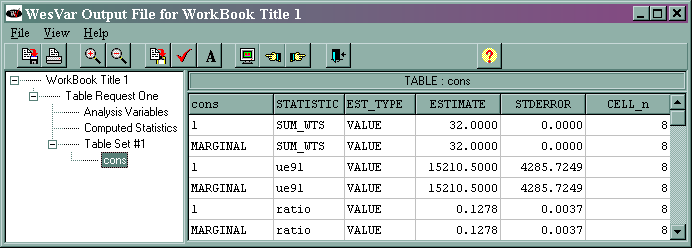
Part of the output is given below.
The marginal sum_wts value of 32 is the estimated population total. The marginal ue91 value of 15210.5 is the estimated total of the variable ue91, and its standard error is 4285.7249. The marginal ratio value of 0.1278 is the estimated ratio of ue91/lab91, and its standard error is 0.0037. The output regarding the median has been omitted. The results from WesVar differ from those given in the text. We suspect that this is due to a difference in the algorithms used by the different statistical packages.


