Version info: Code for this page was tested in R version 3.3.1 (2016-06-21)

 On: 2016-08-26

With: doBy 4.5-14; MplusAutomation 0.6-4; knitr 1.12.3; Hmisc 3.17-4; Formula 1.2-1; fitdistrplus 1.0-7; reshape2 1.4.1; ggplot2 2.1.0; memisc 0.99.7-1; lattice 0.20-33; plyr 1.8.3; JMbayes 0.7-9; survival 2.39-4; nlme 3.1-128; MASS 7.3-45; lme4 1.1-11; Matrix 1.2-6
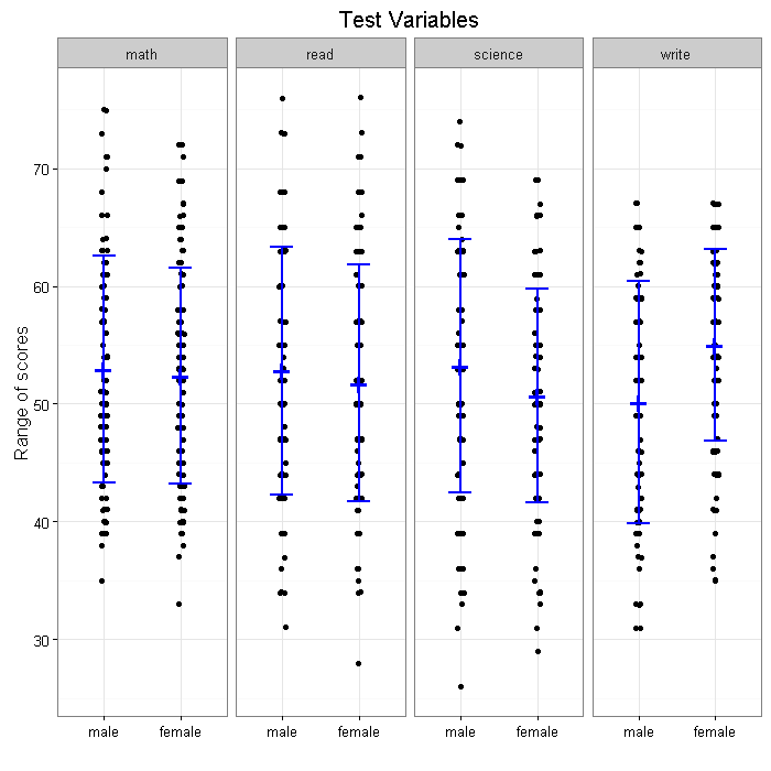
Let’s say that we want to produce a graph of scores for males and
females broken down by subject, with the raw data and mean and
standard error bars in ggplot2.
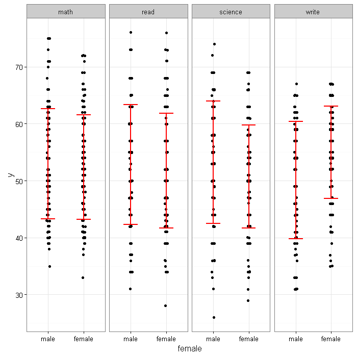
There are four panels for four test score variables, math, read, science and
write from 200 students. Each panel displays by gender an error bar overlaying
jittered data points. We will show how to achieve this goal by steps using
ggplot2. The data set for the example is hsb2 which can be downloaded from
our server as shown below. For easily getting the statistics by group, we have
used a package called “doBy“,
library(ggplot2)
library(doBy)

hsb2 <- read.table('https://stats.idre.ucla.edu/stat/data/hsb2.csv', header=TRUE, sep=",")
hsb2$female <- factor(hsb2$female, labels = c("male", "female"))
Step 1. We make a data set in long format, so test scores are stacked.
# collecting variables of interest for reshaping the data to long
small <- hsb2[, c("write", "math", "read", "science", "female")]

long <- reshape(small, varying=c("write", "math", "read", "science"),
  new.row.names = (1:800), times = c("write", "math", "read", "science"),
  v.names="y", direction="long", timevar="subject")
head(long[order(long$id),], n=8)
##     female subject  y id
## 1     male   write 52  1
## 201   male    math 41  1
## 401   male    read 57  1
## 601   male science 47  1
## 2   female   write 59  2
## 202 female    math 53  2
## 402 female    read 68  2
## 602 female science 63  2
Step 2. We create a data set containing summary statistics by gender and by subject using the summaryBy function from the package doBy.
(a <- summaryBy(y ~ female + subject , long, FUN = c(mean, sd)))
##   female subject y.mean  y.sd
## 1   male    math   52.9  9.66
## 2   male    read   52.8 10.51
## 3   male science   53.2 10.73
## 4   male   write   50.1 10.31
## 5 female    math   52.4  9.15
## 6 female    read   51.7 10.06
## 7 female science   50.7  9.04
## 8 female   write   55.0  8.13
Now we can try to make some graphs. We display all the intermediate graphs below together with R code.
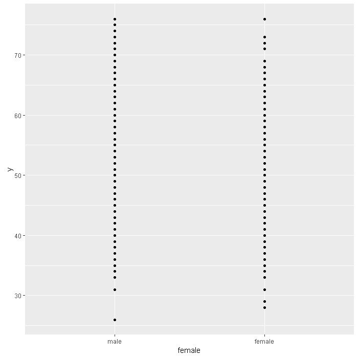
#creating a ggplot object
p <- ggplot(long, aes(y=y, x=female))
p + geom_point()
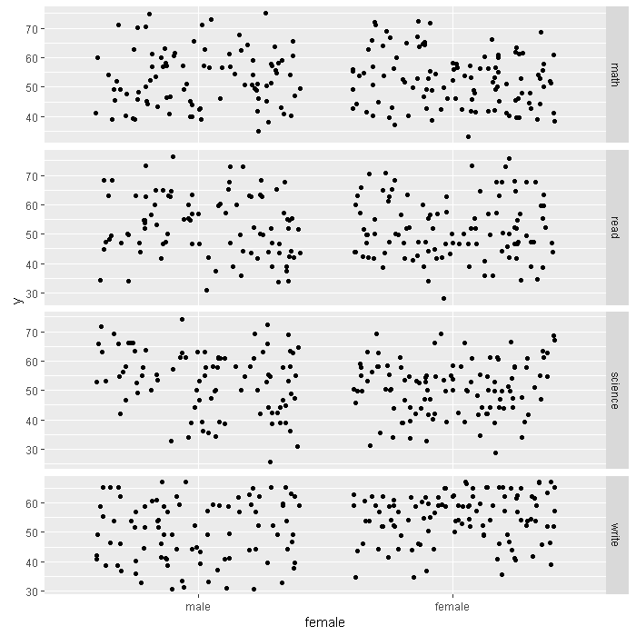
# jittered points and adding a facet
p +
  geom_jitter() +
  facet_grid(subject ~ ., scales="free", space="free")
# reducing jitter and changing to vertical
p +
  geom_jitter(position=position_jitter(w=0.1, h=0.1)) +
  facet_grid(. ~ subject, scales="free",  space="free")

# changing the background to white
p +
  geom_jitter(position=position_jitter(w=0.1, h=0.1)) +
  facet_grid(.~ subject, scales="free", space="free") +
  theme_bw()

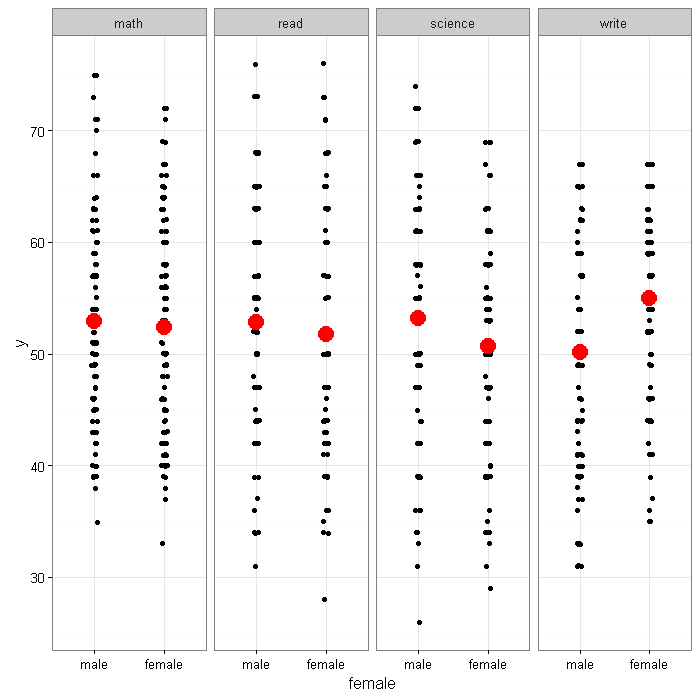
# adding a layer using the summary data set
p +
  geom_jitter(position=position_jitter(w=0.1, h=0.1)) +
  geom_point(data=a, aes(x = female, y = y.mean), size=5, color="red") +
  facet_grid(. ~ subject, scales="free",  space="free") +
  theme_bw()
#alternate code that does not require new dataset
#p +
#  geom_jitter(position=position_jitter(w=0.1, h=0.1)) +
#  stat_summary(fun.y="mean", geom="point", size=5, color="red") +
#  facet_grid(. ~ subject, scales="free",  space="free") +
#  theme_bw()
# add error bar with user-defined limits
p +
  geom_jitter(position=position_jitter(w=0.1, h=0.1)) +
  geom_errorbar(data = a, mapping = aes(x = female, y = y.mean, ymin = y.mean - y.sd, ymax = y.mean + y.sd), size=1, color="red", width=.4) +
  facet_grid(. ~ subject, scales="free", space="free") +
  theme_bw()
#alternate code that does not require new dataset
#p +
#  geom_jitter(position=position_jitter(w=0.1, h=0.1)) +
#  stat_summary(aes(x=female, y=y), geom="errorbar", fun.data="mean_sdl",
#               fun.args=list(mult=1), size=1, color="red", width=.4) +
#  facet_grid(. ~ subject, scales="free", space="free") +
#  theme_bw()
# adding the horizontal line across median, no jitter
# using a different color
p +
  geom_point()+
  geom_errorbar(data = a, mapping = aes(x = female, y = y.mean,
    ymin = y.mean - y.sd, ymax = y.mean + y.sd),
    size=.9, color="Blue", width=.3)+
  geom_point(data = a, mapping = aes(x =female, y= y.mean),
    size=8, color="Blue", shape="+") +
  facet_grid(. ~ subject, scales="free", space="free") +
  labs(title = "Test Variables") +
  theme_bw() +
  xlab('') +
  ylab('Range of scores')
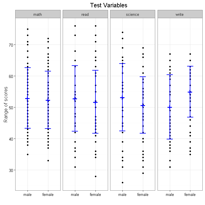
# final product
p +
  geom_jitter(position=position_jitter(w=0.1, h=0.1), size=1.5) +
  geom_errorbar(data = a, mapping = aes(x = female, y = y.mean,
    ymin = y.mean -y.sd, ymax = y.mean + y.sd),
    size=.9, color="Blue", width=.3) +
  geom_point(data = a, mapping = aes(x =female, y= y.mean),
    size=8, color="Blue",  shape="+") +
  facet_grid(.~ subject, scales="free", space="free") +
  labs(title = "Test Variables") +
  theme_bw() +
  xlab('') +
  ylab('Range of scores')