Version info: Code for this page was tested in R Under development (unstable) (2012-07-05 r59734)

 On: 2012-08-08

With: knitr 0.6.3
It is not uncommon to wish to run an analysis in R in which one analysis step is repeated with a different variable each time. Often, the easiest way to list these variable names is as strings. The code below gives an example of how to loop through a list of variable names as strings and use the variable name in a model. A single string is generated using paste that contains the code for the model, and then we use eval and parse to evaluate this string as code.
hsb2 <- read.csv("https://stats.idre.ucla.edu/stat/data/hsb2.csv")
names(hsb2)
##  [1] "id"      "female"  "race"    "ses"     "schtyp"  "prog"    "read"
##  [8] "write"   "math"    "science" "socst"
varlist <- names(hsb2)[8:11]

models <- lapply(varlist, function(x) {
    lm(substitute(read ~ i, list(i = as.name(x))), data = hsb2)
})

## look at the first element of the list, model 1
models[[1]]
##
## Call:
## lm(formula = substitute(read ~ i, list(i = as.name(x))), data = hsb2)
##
## Coefficients:
## (Intercept)        write
##      18.162        0.646
##
## apply summary to each model stored in the list, models
lapply(models, summary)
## [[1]]
##
## Call:
## lm(formula = substitute(read ~ i, list(i = as.name(x))), data = hsb2)
##
## Residuals:
##     Min      1Q  Median      3Q     Max
## -19.857  -5.898  -0.857   5.580  24.270
##
## Coefficients:
##             Estimate Std. Error t value Pr(>|t|)
## (Intercept)  18.1622     3.3072    5.49  1.2e-07 ***
## write         0.6455     0.0617   10.47  < 2e-16 ***
## ---
## Signif. codes:  0 '***' 0.001 '**' 0.01 '*' 0.05 '.' 0.1 ' ' 1
##
## Residual standard error: 8.25 on 198 degrees of freedom
## Multiple R-squared: 0.356,	Adjusted R-squared: 0.353
## F-statistic:  110 on 1 and 198 DF,  p-value: <2e-16
##
##
## [[2]]
##
## Call:
## lm(formula = substitute(read ~ i, list(i = as.name(x))), data = hsb2)
##
## Residuals:
##     Min      1Q  Median      3Q     Max
## -17.239  -4.870  -0.363   4.680  23.559
##
## Coefficients:
##             Estimate Std. Error t value Pr(>|t|)
## (Intercept)  14.0725     3.1158    4.52  1.1e-05 ***
## math          0.7248     0.0583   12.44  < 2e-16 ***
## ---
## Signif. codes:  0 '***' 0.001 '**' 0.01 '*' 0.05 '.' 0.1 ' ' 1
##
## Residual standard error: 7.7 on 198 degrees of freedom
## Multiple R-squared: 0.439,	Adjusted R-squared: 0.436
## F-statistic:  155 on 1 and 198 DF,  p-value: <2e-16
##
##
## [[3]]
##
## Call:
## lm(formula = substitute(read ~ i, list(i = as.name(x))), data = hsb2)
##
## Residuals:
##     Min      1Q  Median      3Q     Max
## -23.379  -5.980   0.155   5.780  18.714
##
## Coefficients:
##             Estimate Std. Error t value Pr(>|t|)
## (Intercept)  18.3945     3.0161     6.1  5.5e-09 ***
## science       0.6526     0.0571    11.4  < 2e-16 ***
## ---
## Signif. codes:  0 '***' 0.001 '**' 0.01 '*' 0.05 '.' 0.1 ' ' 1
##
## Residual standard error: 7.98 on 198 degrees of freedom
## Multiple R-squared: 0.397,	Adjusted R-squared: 0.394
## F-statistic:  130 on 1 and 198 DF,  p-value: <2e-16
##
##
## [[4]]
##
## Call:
## lm(formula = substitute(read ~ i, list(i = as.name(x))), data = hsb2)
##
## Residuals:
##     Min      1Q  Median      3Q     Max
## -23.396  -6.437  -0.315   5.669  18.669
##
## Coefficients:
##             Estimate Std. Error t value Pr(>|t|)
## (Intercept)  21.1259     2.8440    7.43  3.2e-12 ***
## socst         0.5935     0.0532   11.16  < 2e-16 ***
## ---
## Signif. codes:  0 '***' 0.001 '**' 0.01 '*' 0.05 '.' 0.1 ' ' 1
##
## Residual standard error: 8.05 on 198 degrees of freedom
## Multiple R-squared: 0.386,	Adjusted R-squared: 0.383
## F-statistic:  125 on 1 and 198 DF,  p-value: <2e-16
##
##
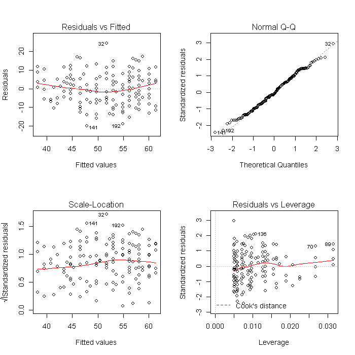
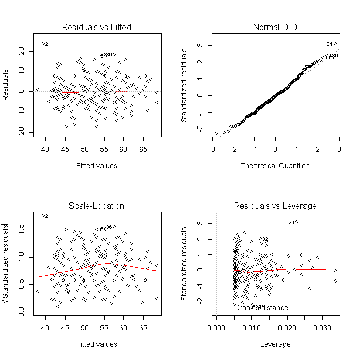
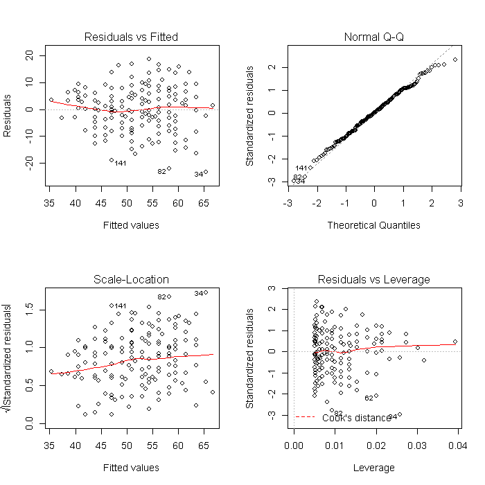
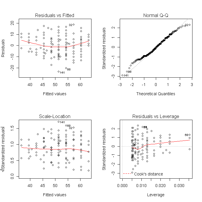
Using a list is also convenient because it makes other common tasks straightforward. For example, we can create all of the diagnostic model plots quickly. First we set the graphical parameters so that each plot window contains 4 (2 x 2) plots, and set ask = TRUE so that R will ask before changing graphs (otherwise the plots would flash before your eyes before you could look at them). The results will look like this:
par(mfrow = c(2, 2))
invisible(lapply(models, plot))


