Version info: Code for this page was tested in R Under development (unstable) (2012-07-05 r59734)

 On: 2012-08-08

With: knitr 0.6.3
This shows and documents the code used to simulate the Hospital, Doctor, Patient (HDP) dataset. This dataset has a three-level, hierarchical structure with patients nested within doctors within hospitals. The purpose of this simulation is not to do a simulation study, but rather to create a rich dataset that can be used to show a variety of analytic techniques. However, the principles used in this simulation could be easily abstracted and a handful or parameters varied to do a simulation study.
The simulation is broken down into sections. The first is the setup and creation of the IDs and all predictor variables across the three levels. Then there is a separate section for each outcome.
- Setup
- Tumor size
- CO2
- Pain
- Wound
- Mobility
- Number of tumors (right censored)
- Number of self-administered morphine doses
- Cancer in remission
- Proportion of optimal lung capacity
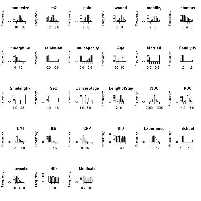
The study is meant to be a large study of lung cancer outcomes across multiple doctors and sites. Here is a list of all the outcomes and their predictors at each level. Note that there are cross level interactions, and not all predictors are necessarily significant. Being listed as a predictor merely means the true coefficient was not zero. When Doctor ID (DID) or Hospital ID (HID) is specified, it means random intercepts. Random slopes are indicated in parentheses. Also note that there are some interactions with no simple main effects (or true value for simple main effects 0). That is, the true model includes interactions without their respective main effects. Put differently, sometimes the product of variables has an effect, but they do not have an additive effect. Characteristics of the predictors are described under the setup. Distributions of all variables are graphed. Please see the notes and code below for additional details.
| Variable | Type | L1 Predictors | L2 Predictors | L3 Predictors |
| Tumor size | Continuous, Gaussian (correlated with CO2, multivariate multilevel candidate) |
|
|
|
| CO2 (percents) | Continuous, Gaussian (correlated with Tumor size, multivariate multilevel candidate) |
|
|
|
| Pain | Continuous, Gaussian cut to be integer ranging from 1 to 10 |
|
|
|
| Wound | Continuous, Gaussian cut to be integer ranging from 1 to 10 |
|
|
|
| Mobility | Continuous, Gaussian cut to be integer ranging from 1 to 10 |
|
|
|
| Number of tumors (right censored) | Count, Poisson, right censored at 9 |
|
|
|
| Number of self-administered morphine doses | Count, Poisson, zero-inflated | Zero-inflation (binomial model)
Poisson model
|
Zero-inflation (binomial model)
Poisson model
|
|
| Cancer in remission (TRUE/FALSE) | Dichotomized normal |
|
|
|
| Proportion of optimal lung capacity | Continuous, Beta |
|
|
Setup
First we will load the packages required for the simulation and define function (called dmat) to return a structural design matrix (hence the name, dmat) given a vector, i where the number of elements (the length of i) are the number of groups and the value of each element of i is the number of subunits in each group. For example, for doctors within hospitals, the length of i would be the number of hospitals, and if the value of the first element was 10, it would mean there were 10 doctors within the first hospital. This is necessary because the simulation is designed to have varying number of doctors within each hospital and patients within each doctor to more closely approximate what real life data tend to look like. There is also a little helper function (hgraph) to easily create histograms for an entire dataset, lay them out in a plot matrix, and title them reasonably.
require(compiler) # to compile our function
require(lme4) # mixed models
require(MASS) # for multivariate normal function
require(corpcor) # to make a matrix positive definite
dmat <- cmpfun(function(i) {
    j <- length(i)
    n <- sum(i)
    index <- cbind(start = cumsum(c(1, i[-j])), stop = cumsum(i))
    H <- matrix(0, nrow = n, ncol = j)
    for (i in 1:j) {
        H[index[i, 1]:index[i, 2], i] <- 1L
    }
    return(H)
})

r <- cmpfun(function(n, mu, sigma, data) {
    dmat(n) %*% rnorm(length(n), mu, sigma) * data
})

logit <- cmpfun(function(xb) 1/(1 + exp(-xb)))

mycut <- cmpfun(function(x, p) {
    cut(x = x, breaks = quantile(x, probs = p), labels = FALSE, include.lowest = TRUE)
})

hgraph <- cmpfun(function(data) {
    oldpar <- par(no.readonly = TRUE)
    on.exit(par(oldpar))

    n <- ncol(data)
    ncol <- ceiling(sqrt(n))
    nrow <- ceiling(n/ncol)
    par(mfrow = c(nrow, ncol))
    if (!is.null(colnames(data))) {
        i <- colnames(data)
    } else {
        i <- seq(from = 1, to = n)
    }
    out <- lapply(i, function(x) {
        if (is.numeric(data[, x])) {
            hist(data[, x], main = x, xlab = "")
        } else barplot(table(data[, x]), main = x, xlab = "", ylab = "Frequency")
    })
    return(invisible(out))
})
Now we can set some of the simulation parameters. Not everything is set upfront
## seed for simulation parameters
set.seed(1)

# total number of hospitals
k <- 35

# number of doctors within each hospital
n <- sample(8:15, size = k, TRUE)
# total number of doctors
j <- sum(n)


# number of patients within each doctor
N <- sample(2:40, size = j, TRUE)
# total number of patients
i <- sum(N)

mu <- list(int = 0, experience = 18, cont = c(Age = 5.1, Married = 0,
    FamilyHx = 0, SmokingHx = 0, Sex = 0, CancerStage = 0, LengthofStay = 6,
    WBC = 6000, RBC = 5), bounded = c(BMI = 5.5, IL6 = 4, CRP = 5))


R <- diag(9)
rownames(R) <- names(mu$cont)
R[1, 2] <- 0.3
R[1, 4] <- 0.3
R[1, 6] <- 0.5
R[1, 7] <- 0.5
R[2, 6] <- -0.2
R[2, 7] <- -0.4
R[2, 8] <- 0.25
R[3, 4] <- -0.5
R[3, 6] <- 0.3
R[3, 7] <- 0.3
R[4, 5] <- 0.3
R[4, 6] <- 0.7
R[4, 7] <- 0.5
R[6, 7] <- 0.5
R[7, 8] <- -0.3
R[8, 9] <- -0.1
R[lower.tri(R)] <- t(R)[lower.tri(t(R))]
(R <- cov2cor(make.positive.definite(R)))
##                   [,1]      [,2]      [,3]      [,4]      [,5]      [,6]
## Age           1.000000  0.283565  0.021670  0.316729 -7.13e-03  0.465972
## Married       0.283565  1.000000 -0.021195 -0.026969  6.97e-03 -0.173915
## FamilyHx      0.021670 -0.021195  1.000000 -0.429945 -1.19e-02  0.252758
## SmokingHx     0.316729 -0.026969 -0.429945  1.000000  2.75e-01  0.620402
## Sex          -0.007127  0.006971 -0.011950  0.275264  1.00e+00  0.011952
## CancerStage   0.465972 -0.173915  0.252758  0.620402  1.20e-02  1.000000
## LengthofStay  0.472200 -0.374636  0.260246  0.440067  1.00e-02  0.514992
## WBC          -0.001975  0.250344 -0.003312 -0.004214  1.09e-03  0.003313
## RBC          -0.000165  0.000162 -0.000277 -0.000353  9.12e-05  0.000277
##                   [,7]     [,8]      [,9]
## Age           0.472200 -0.00198 -1.65e-04
## Married      -0.374636  0.25034  1.62e-04
## FamilyHx      0.260246 -0.00331 -2.77e-04
## SmokingHx     0.440067 -0.00421 -3.53e-04
## Sex           0.010021  0.00109  9.12e-05
## CancerStage   0.514992  0.00331  2.77e-04
## LengthofStay  1.000000 -0.29332  2.33e-04
## WBC          -0.293321  1.00000 -1.00e-01
## RBC           0.000233 -0.09996  1.00e+00
p <- list(school = 0.25, sex = 0.4, married = 0.6, familyhx = 0.2,
    smokehx = c(0.2, 0.2, 0.6), stage = c(0.3, 0.4, 0.2, 0.1))
Now we will generate some hospital level data (L3). There is a random intercept and a variable (Medicaid) that is the proportion of cases that rely on Medicaid at a given hospital. To expand the hospital level variables to have the same dimensions as the patient level, we post multiply the design matrices for both the lower levels by the effects (stored in the matrix b).
set.seed(84361)

## hospital variables
b <- cbind(HID = 1:k, Hint = rnorm(k, mean = mu$int, sd = 1), Medicaid = runif(k,
    min = 0.1, max = 0.85))
H <- dmat(N) %*% dmat(n) %*% b

## View the first few rows
head(H)
##      HID  Hint Medicaid
## [1,]   1 -1.92    0.606
## [2,]   1 -1.92    0.606
## [3,]   1 -1.92    0.606
## [4,]   1 -1.92    0.606
## [5,]   1 -1.92    0.606
## [6,]   1 -1.92    0.606
## View a graph of the distributions
hgraph(H)
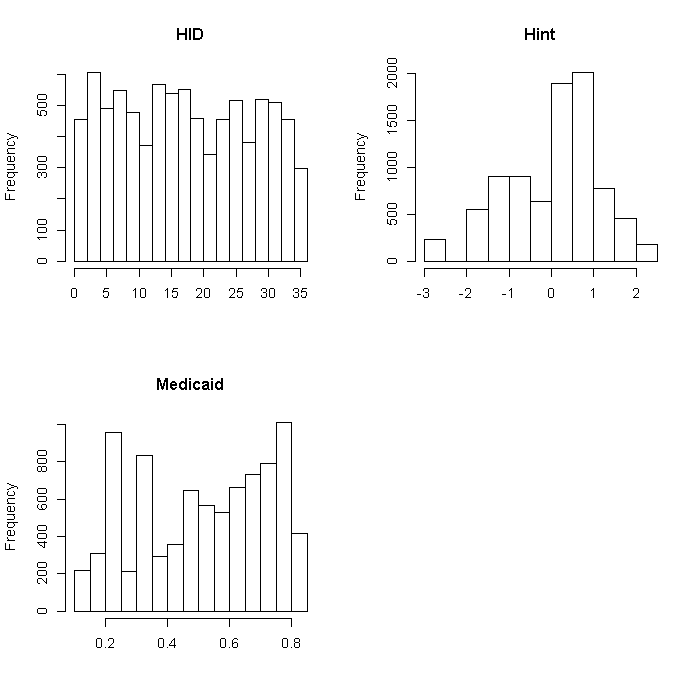
Now we will generate the doctor level (L2) predictors. There is an ID (DID), a random intercept variable, an experience variable (years in practice as a doctor), a school variable (whether the school doctors trained at was high quality or not), and a lawsuits variable (number of lawsuits). To expand the doctor level variables to have the same dimensions as the patient level, we post multiply the design matrix by the effects (stored in the matrix b).
set.seed(50411)
## doctor variables
b <- cbind(DID = 1:j, Dint = rnorm(j, mean = mu$int, sd = 1), Experience = experience <- floor(rnorm(j,
    mean = mu$experience, sd = 4)), School = school <- rbinom(j, 1, prob = p$school),
    Lawsuits = rpois(j, pmax(experience - 8 * school, 0)/8))
D <- dmat(N) %*% b

## View the first few rows
head(D)
##      DID  Dint Experience School Lawsuits
## [1,]   1 -2.76         25      0        3
## [2,]   1 -2.76         25      0        3
## [3,]   1 -2.76         25      0        3
## [4,]   1 -2.76         25      0        3
## [5,]   1 -2.76         25      0        3
## [6,]   1 -2.76         25      0        3
## View a graph of the distributions
hgraph(D)
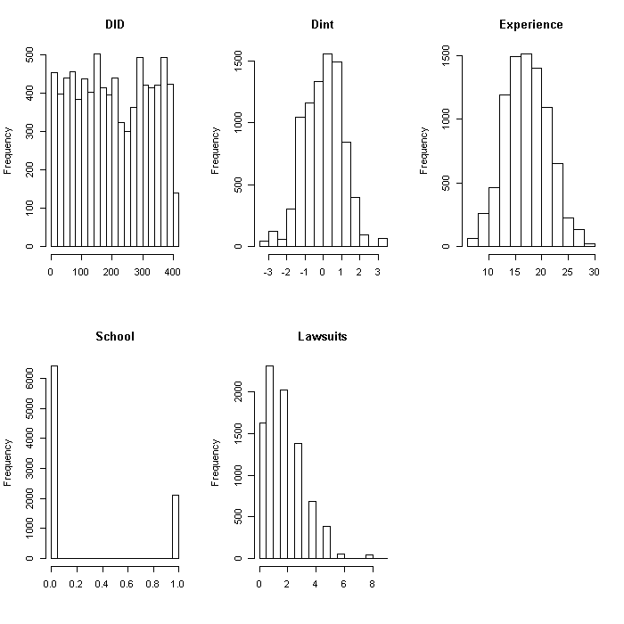
Now we will generate some patient level data (L1). There are nine predictors.
- Age: continuous in years but recorded at a higher degree of accuracy
- Married: binary, married/living with partner or single.
- Family Hx: binary (yes/no), does the patient have a family history (Hx) of cancer?
- Smoking Hx: categorical with three levels, current smoker, former smoker, never smoked
- Sex: binary (female/male)
- Cancer stage: categorical with four levels, stages 1-4
- Length of stay: count number of days patients stayed in the hospital after surgery
- WBC: continuous, white blood count. Roughly 3,000 is low, 10,000 is middle, and 30,000 per microliter is high.
- RBC: continuous, red blood count.
- BMI: continuous, body mass index given by the formula (frac{kg}{meters^2})
- IL6: continuous, interleukin 6, a proinflammatory cytokine commonly examined as an indicator of inflammation, cannot be lower than zero
- CRP: continuous, C-reactive protein, a protein in the blood also used as an indicator of inflammation. It is also impacted by BMI.
The means and spread of Age, BMI, IL6, CRP, and Cancer Stage were roughly based on descriptives from this article Fatigue and sleep quality are associated with changes in inflammatory markers in breast cancer patients undergoing chemotherapy by Lianqi Liua and colleagues.
set.seed(38983)

## continuous variables
Xc <- as.data.frame(cbind(mvrnorm(n = i, mu = rep(0, 9), Sigma = R),
  sapply(mu$bounded, function(k) rchisq(n = i, df = k))))

Xc <- within(Xc, {
  Age <- ((Age/1.6) + mu$cont["Age"]) * 10
  Married <- mycut(Married, c(0, 1-p$married, 1)) - 1
  FamilyHx <- mycut(FamilyHx, c(0, 1-p$familyhx, 1)) - 1
  SmokingHx <- factor(mycut(SmokingHx, c(0, cumsum(p$smokehx))))
  Sex <- mycut(Sex, c(0, 1-p$sex, 1)) - 1
  CancerStage <- factor(mycut(CancerStage, c(0, cumsum(p$stage))))
  LengthofStay <- floor(LengthofStay + mu$cont["LengthofStay"])
  WBC <- ((WBC/.001) + mu$cont["WBC"])
  RBC <- ((RBC/3.5) + mu$cont["RBC"])
  BMI <- pmin(BMI * 2 + 18, 58)
})


## first few rows and histograms
head(Xc)
##    Age Married FamilyHx SmokingHx Sex CancerStage LengthofStay  WBC  RBC
## 1 65.0       0        0         2   1           2            6 6088 4.87
## 2 53.9       0        0         2   0           2            6 6700 4.68
## 3 53.3       1        0         3   0           2            5 6043 5.01
## 4 41.4       0        0         2   1           1            5 7163 5.27
## 5 46.8       0        0         3   1           2            6 6443 4.98
## 6 51.9       1        0         3   1           1            5 6801 5.20
##    BMI   IL6   CRP
## 1 24.1  3.70 8.086
## 2 29.4  2.63 0.803
## 3 29.5 13.90 4.034
## 4 21.6  3.01 2.126
## 5 29.8  3.89 1.349
## 6 27.1  1.42 2.195
hgraph(Xc)
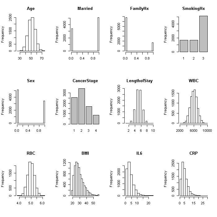
For the purposes of simulating the outcomes, we also create a number of interactions and dummy variables to code the categorical variables. These are not maintained in the final dataset. Finally, we combine the matrices from all the levels. We create two matrices, one of the raw data, the other of the dummy coded data with interactions to use for simulating the outcomes.
## create dummies and drop the intercept
Xmdummy <- model.matrix(~ 1 + SmokingHx + CancerStage, data = Xc)[, -1]

X <- cbind(Xc[, -c(4,6)], Xmdummy,
  "Sex:Married" = Xc[, "Sex"] * Xc[, "Married"],
  "IL6:CRP" = Xc[, "IL6"] * Xc[, "CRP"],
  "BMI:FamilyHx" = Xc[, "BMI"] * Xc[, "FamilyHx"],
  "SmokingHx2:FamilyHx" = Xmdummy[, "SmokingHx2"] * Xc[, "FamilyHx"],
  "SmokingHx3:FamilyHx" = Xmdummy[, "SmokingHx3"] * Xc[, "FamilyHx"],
  "SmokingHx2:Age" = Xmdummy[, "SmokingHx2"] * Xc[, "Age"],
  "SmokingHx3:Age" = Xmdummy[, "SmokingHx3"] * Xc[, "Age"],
  "Experience:CancerStage2" = D[, "Experience"] * Xmdummy[, "CancerStage2"],
  "Experience:CancerStage3" = D[, "Experience"] * Xmdummy[, "CancerStage3"],
  "Experience:CancerStage4" = D[, "Experience"] * Xmdummy[, "CancerStage4"])

## Final data
mldat <- data.frame(Xc, D, H)
mldat <- mldat[, -which(colnames(mldat) %in% c("Dint", "Hint"))]

mldat <- within(mldat, {
  Sex <- factor(Sex, labels = c("female", "male"))
  FamilyHx <- factor(FamilyHx, labels = c("no", "yes"))
  SmokingHx <- factor(SmokingHx, labels = c("current", "former", "never"))
  CancerStage <- factor(CancerStage, labels = c("I", "II", "III", "IV"))
  School <- factor(School, labels = c("average", "top"))
  DID <- factor(DID)
  HID <- factor(HID)
})

## view histogram matrix
hgraph(mldat)
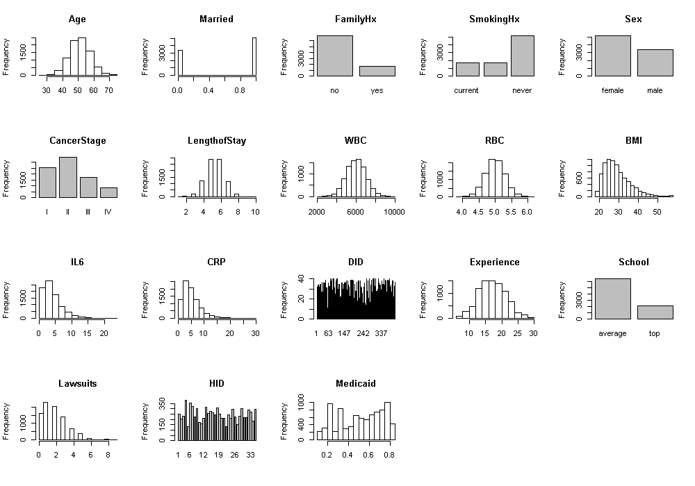
## Final for simulation
dat <- cbind(X, D, H)
dat <- as.matrix(dat[, -which(colnames(dat) %in% c("DID", "HID"))])
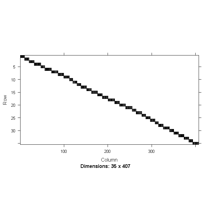
We can look at the cross tabs of the doctor and hospital ID, which clearly shows the nested structure. We will also label the final data set.
image(t(xtabs(~DID + HID, data = mldat, sparse = TRUE)), asp = 0.5)
## View a summary
summary(mldat)
##       Age          Married    FamilyHx     SmokingHx        Sex
##  Min.   :26.3   Min.   :0.0   no :6820   current:1705   female:5115
##  1st Qu.:46.7   1st Qu.:0.0   yes:1705   former :1705   male  :3410
##  Median :50.9   Median :1.0              never  :5115
##  Mean   :51.0   Mean   :0.6
##  3rd Qu.:55.3   3rd Qu.:1.0
##  Max.   :74.5   Max.   :1.0
##
##  CancerStage  LengthofStay        WBC            RBC            BMI
##  I  :2558    Min.   : 1.00   Min.   :2131   Min.   :3.92   Min.   :18.4
##  II :3409    1st Qu.: 5.00   1st Qu.:5323   1st Qu.:4.80   1st Qu.:24.2
##  III:1705    Median : 5.00   Median :6007   Median :4.99   Median :27.7
##  IV : 853    Mean   : 5.49   Mean   :5998   Mean   :5.00   Mean   :29.1
##              3rd Qu.: 6.00   3rd Qu.:6663   3rd Qu.:5.19   3rd Qu.:32.5
##              Max.   :10.00   Max.   :9776   Max.   :6.06   Max.   :58.0
##
##       IL6             CRP             DID         Experience
##  Min.   : 0.04   Min.   : 0.05   69     :  40   Min.   : 7.0
##  1st Qu.: 1.93   1st Qu.: 2.70   76     :  40   1st Qu.:15.0
##  Median : 3.34   Median : 4.33   86     :  40   Median :18.0
##  Mean   : 4.02   Mean   : 4.97   104    :  40   Mean   :17.6
##  3rd Qu.: 5.41   3rd Qu.: 6.60   258    :  40   3rd Qu.:21.0
##  Max.   :23.73   Max.   :28.74   271    :  40   Max.   :29.0
##                                  (Other):8285
##      School        Lawsuits         HID          Medicaid
##  average:6405   Min.   :0.00   4      : 377   Min.   :0.142
##  top    :2120   1st Qu.:1.00   6      : 356   1st Qu.:0.337
##                 Median :2.00   7      : 322   Median :0.522
##                 Mean   :1.87   13     : 312   Mean   :0.513
##                 3rd Qu.:3.00   18     : 307   3rd Qu.:0.708
##                 Max.   :9.00   9      : 302   Max.   :0.819
##                                (Other):6549
b <- as.data.frame(rbind(
  'Age' = c(1, 1, 0, 0, 1, 8, .8, -1, -1, 0),
  'Married' = c(0, 0, 0, 1, 0, 0, 0, 0, 0, 0),
  'FamilyHx' = c(1, 1, 0, 0, 0, -8, 0, 0, -5, 0),
  'Sex' = c(0, 0, -1, 1, 0, 0, 0, -1, 0, 0),
  'LengthofStay' = c(0, 0, 0, 0, 0, 0, 0, .9, 0, 0),
  'WBC' = c(0, 0, 0, 0, 0, 0, 0, 0, 0, 0),
  'RBC' = c(0, 0, 0, 0, 0, 0, 0, 0, 0, -2),
  'BMI' = c(0, 0, 0, 0, 1, 1, 0, 0, 0, 0),
  'IL6' = c(0, 0, 1, 0, 0, 3.2, 0, 0, -1, 0),
  'CRP' = c(0, 0, 1, 0, 0, 5, 0, 0, -.8, 0),
  'SmokingHx2' = c(-1, -1, 0, 0, 0, -2, -2, 0, 0, 0),
  'SmokingHx3' = c(-2, -2, 0, 0, 0, -10, -4, 0, 0, 0),
  'CancerStage2' = c(1, 1, 0, 0, 0, .5, 2, 1, -1, 0),
  'CancerStage3' = c(1.5, 1.5, 0, 0, 0, 1, 4, 2, -3, 0),
  'CancerStage4' = c(2, 2, 0, 0, 0, 2, 6, 3, -6, 0),
  'Sex:Married' = c(0, 0, 0, 4, 0, 0, 0, 0, 0, 0),
  'IL6:CRP' = c(0, 0, 3, 0, 0, 0, 0, 0, 0, 5),
  'BMI:FamilyHx' = c(0, 0, 0, 0, 0, 60, 0, 0, 0, 0),
  'SmokingHx2:FamilyHx' = c(0, 0, 0, 0, 0, 0, 0, 0, 0, -.5),
  'SmokingHx3:FamilyHx' = c(0, 0, 0, 0, 0, 0, 0, 0, 0, -5),
  'SmokingHx2:Age' = c(-4, -4, 0, 0, 0, 0, 0, 0, 0, 0),
  'SmokingHx3:Age' = c(-8, -8, 0, 0, 0, 0, 0, 0, 0, 0),
  'Experience:CancerStage2' = c(0, 0, 0, 0, 0, 4, 0, 0, 0, 0),
  'Experience:CancerStage3' = c(0, 0, 0, 0, 0, 16, 0, 0, 0, 0),
  'Experience:CancerStage4' = c(0, 0, 0, 0, 0, 40, 0, 0, 0, 0),
  'Dint' = c(3, 3, 3, 3, 3, 20, 8, 10, 5, 10),
  'Experience' = c(0, 0, 0, -5, -3, 0, 0, 0, 3, 2),
  'School' = c(0, 0, 0, 0, 2, 0, 0, 0, 0, 1),
  'Lawsuits' = c(0, 0, 0, 0, -2, 0, 0, 0, 0, 0),
  'Hint' = c(0, 0, 0, 4, 5, 40, 0, 0, 6, 0),
  'Medicaid' = c(0, 0, 0, 0, 3, 0, 0, 0, 0, 0)
))
b <- b / apply(dat, 2, sd)
colnames(b) <- c("tumor", "co2", "pain", "wound", "mobility", "ntumors",
  "zeroinflation", "nmorphine", "remission", "lungcapacity")
Tumor size and CO2
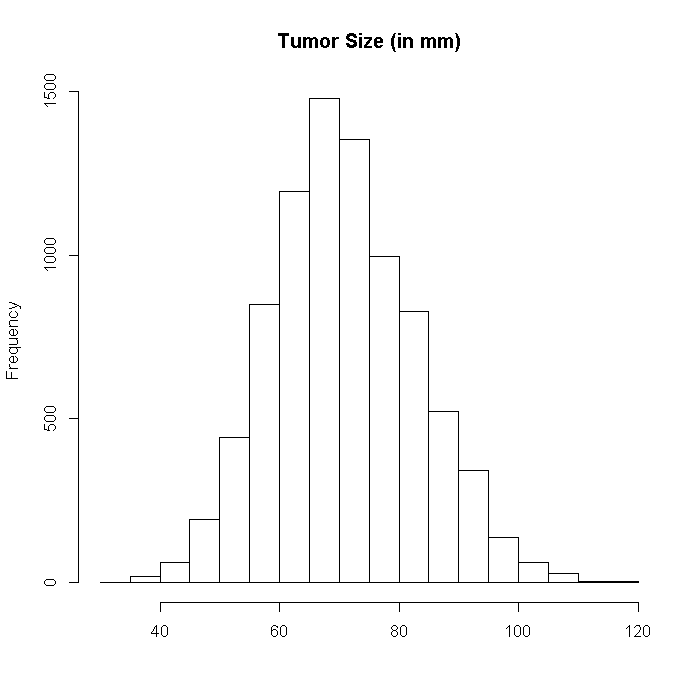
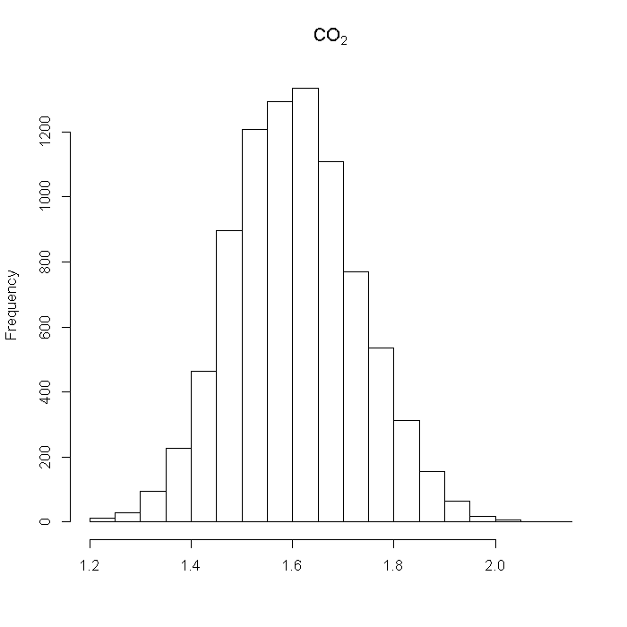
Now we can generate the data for the outcome, tumor size. First we create a vector of the true coefficients, which is premultiplied by the predictor matrix, and then the data will be drawn from a normal distribution with the expectation from our true model. The outcome is the tumor size in millimeters (mm). The outcome is CO2 levels in percents. Tumor size and CO2 are both indicators of disease severity and actually have the same prediction model so are highly correlated. Although they can be analyzed individually, they may also be good candidates for a multivariate, multilevel model.
## Tumor Size
set.seed(82231)
outcome <- data.frame(tumorsize = rnorm(n = i, mean = (dat %*% b$tumor) +
    r(N, 0.8, 0.8, dat[, "LengthofStay"]) + 70, sd = 8))
hist(outcome$tumorsize, xlab = "", main = "Tumor Size (in mm)")
mtumorsize.true <- lmer(outcome$tumorsize ~ Age + FamilyHx + LengthofStay +
    SmokingHx + CancerStage + SmokingHx:Age + (1 | DID) + (0 + LengthofStay |
    DID), data = mldat)
print(mtumorsize.true, correlation = FALSE)
## Linear mixed model fit by REML
## Formula: outcome$tumorsize ~ Age + FamilyHx + LengthofStay + SmokingHx +      CancerStage + SmokingHx:Age + (1 | DID) + (0 + LengthofStay |      DID)
##    Data: mldat
##    AIC   BIC logLik deviance REMLdev
##  60351 60450 -30162    60298   60323
## Random effects:
##  Groups   Name         Variance Std.Dev.
##  DID      (Intercept)  12.284   3.505
##  DID      LengthofStay  0.612   0.782
##  Residual              61.722   7.856
## Number of obs: 8525, groups: DID, 407
##
## Fixed effects:
##                     Estimate Std. Error t value
## (Intercept)          71.1825     1.6330    43.6
## Age                   0.1560     0.0337     4.6
## FamilyHxyes           2.5816     0.2526    10.2
## LengthofStay          0.6749     0.1100     6.1
## SmokingHxformer      -3.0503     2.2919    -1.3
## SmokingHxnever       -5.9769     1.8891    -3.2
## CancerStageII         1.8660     0.2360     7.9
## CancerStageIII        3.6171     0.3038    11.9
## CancerStageIV         6.2087     0.3960    15.7
## Age:SmokingHxformer  -0.1925     0.0463    -4.2
## Age:SmokingHxnever   -0.2708     0.0381    -7.1
## CO2
outcome$co2 <- abs(rnorm(n = i, mean = ((dat %*% b$co2) + r(N, 0.8,
    1, dat[, "LengthofStay"]))/100, sd = 0.08) + 1.6)
hist(outcome$co2, xlab = "", main = bquote(CO[2]))
mco2.true <- lmer(outcome$co2 ~ Age + FamilyHx + LengthofStay + SmokingHx +
    CancerStage + SmokingHx:Age + (1 | DID) + (0 + LengthofStay | DID), data = mldat)
print(mco2.true, correlation = FALSE)
## Linear mixed model fit by REML
## Formula: outcome$co2 ~ Age + FamilyHx + LengthofStay + SmokingHx + CancerStage +      SmokingHx:Age + (1 | DID) + (0 + LengthofStay | DID)
##    Data: mldat
##     AIC    BIC logLik deviance REMLdev
##  -17819 -17720   8924   -17973  -17847
## Random effects:
##  Groups   Name         Variance Std.Dev.
##  DID      (Intercept)  1.18e-03 0.03430
##  DID      LengthofStay 9.24e-05 0.00961
##  Residual              6.29e-03 0.07929
## Number of obs: 8525, groups: DID, 407
##
## Fixed effects:
##                      Estimate Std. Error t value
## (Intercept)          1.619725   0.016482    98.3
## Age                  0.001160   0.000340     3.4
## FamilyHxyes          0.026555   0.002552    10.4
## LengthofStay         0.007466   0.001145     6.5
## SmokingHxformer     -0.037865   0.023140    -1.6
## SmokingHxnever      -0.037073   0.019074    -1.9
## CancerStageII        0.021743   0.002383     9.1
## CancerStageIII       0.038288   0.003068    12.5
## CancerStageIV        0.061546   0.004000    15.4
## Age:SmokingHxformer -0.001694   0.000468    -3.6
## Age:SmokingHxnever  -0.003072   0.000385    -8.0
Pain
## Pain
set.seed(37613)
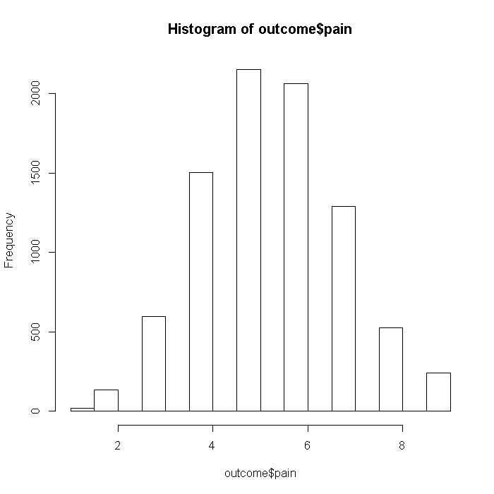
outcome$pain <- rnorm(n = i, mean = (dat %*% b$pain), sd = 6)
outcome$pain <- with(outcome, pmin(pain, quantile(pain, 0.99)))
outcome$pain <- with(outcome, cut(pain, breaks = seq(from = min(pain) -
    0.1, max(pain) + 0.1, length.out = 10), labels = FALSE))
hist(outcome$pain)
mpain.true <- lmer(outcome$pain ~ Sex + IL6 * CRP + (1 | DID), data = mldat)
print(mpain.true, correlation = FALSE)
## Linear mixed model fit by REML
## Formula: outcome$pain ~ Sex + IL6 * CRP + (1 | DID)
##    Data: mldat
##    AIC   BIC logLik deviance REMLdev
##  27499 27548 -13743    27445   27485
## Random effects:
##  Groups   Name        Variance Std.Dev.
##  DID      (Intercept) 0.298    0.546
##  Residual             1.357    1.165
## Number of obs: 8525, groups: DID, 407
##
## Fixed effects:
##             Estimate Std. Error t value
## (Intercept)  4.39534    0.05106    86.1
## Sexmale     -0.40259    0.02628   -15.3
## IL6          0.11017    0.00830    13.3
## CRP          0.09474    0.00701    13.5
## IL6:CRP      0.01613    0.00139    11.6
Wound
## Wound
set.seed(79642)
outcome$wound <- rnorm(n = i, mean = (dat %*% b$wound) + r(N, 3,
    3, dat[, "RBC"]), sd = 4)
outcome$wound <- with(outcome, pmin(wound, quantile(wound, 0.99)))
outcome$wound <- with(outcome, cut(wound, breaks = seq(from = min(wound) -
    0.1, max(wound) + 0.1, length.out = 10), labels = FALSE))
hist(outcome$wound)
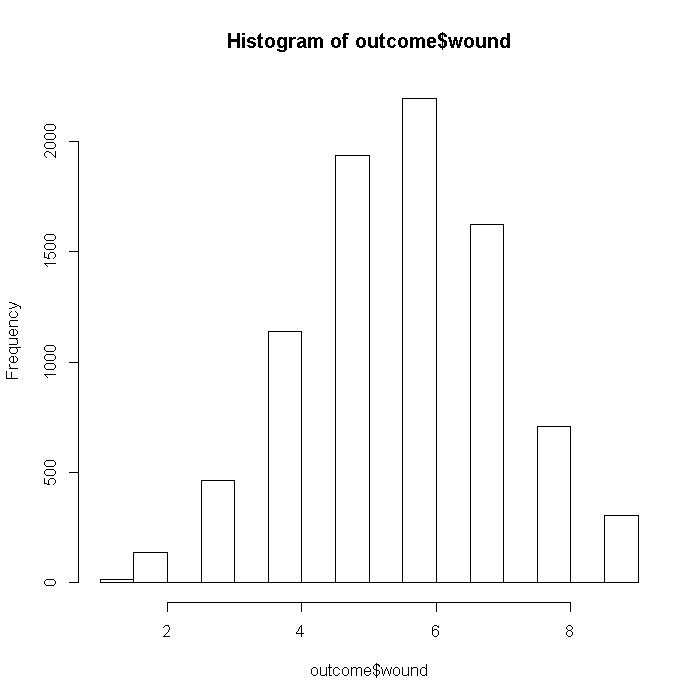
mwound.true <- lmer(outcome$wound ~ Sex * Married + RBC + Experience +
    (1 | DID) + (0 + RBC | DID) + (1 | HID), data = mldat)
print(mwound.true, correlation = FALSE)
## Linear mixed model fit by REML
## Formula: outcome$wound ~ Sex * Married + RBC + Experience + (1 | DID) +      (0 + RBC | DID) + (1 | HID)
##    Data: mldat
##    AIC   BIC logLik deviance REMLdev
##  12313 12384  -6147    12257   12293
## Random effects:
##  Groups   Name        Variance Std.Dev.
##  DID      RBC         0.0555   0.236
##  DID      (Intercept) 0.2880   0.537
##  HID      (Intercept) 0.1029   0.321
##  Residual             0.1928   0.439
## Number of obs: 8525, groups: DID, 407; HID, 35
##
## Fixed effects:
##                 Estimate Std. Error t value
## (Intercept)       6.3203     0.2689    23.5
## Sexmale           0.1691     0.0158    10.7
## Married           0.1911     0.0129    14.9
## RBC               0.2244     0.0207    10.8
## Experience       -0.1183     0.0140    -8.5
## Sexmale:Married   0.7356     0.0203    36.2
Mobility
## Mobility
set.seed(59580)
outcome$mobility <- rnorm(n = i, mean = (dat %*% b$mobility), sd = 3)
outcome$mobility <- with(outcome, pmin(mobility, quantile(mobility,
    0.99)))
outcome$mobility <- with(outcome, cut(mobility, breaks = seq(from = min(mobility) -
    0.1, max(mobility) + 0.1, length.out = 10), labels = FALSE))
hist(outcome$mobility)
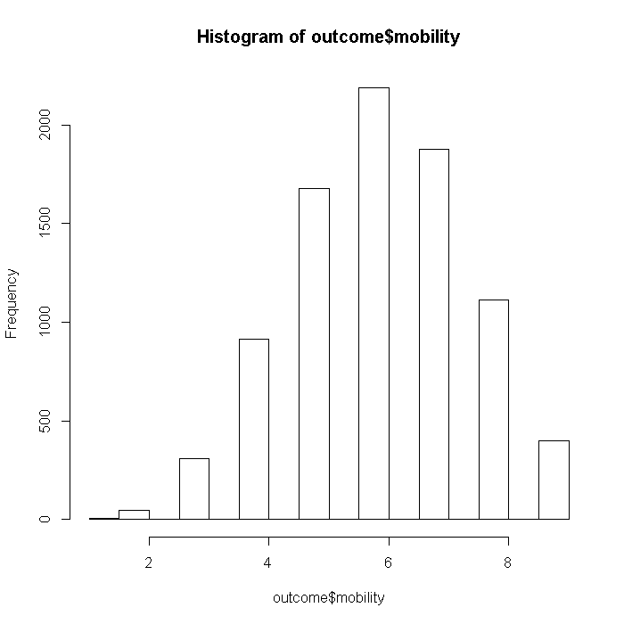
mmobility.true <- lmer(outcome$mobility ~ Age + BMI + Experience +
    School + Lawsuits + Medicaid + (1 | DID) + (1 | HID), data = mldat)
print(mmobility.true, correlation = FALSE)
## Linear mixed model fit by REML
## Formula: outcome$mobility ~ Age + BMI + Experience + School + Lawsuits +      Medicaid + (1 | DID) + (1 | HID)
##    Data: mldat
##    AIC   BIC logLik deviance REMLdev
##  15427 15498  -7704    15364   15407
## Random effects:
##  Groups   Name        Variance Std.Dev.
##  DID      (Intercept) 0.214    0.463
##  HID      (Intercept) 0.690    0.831
##  Residual             0.309    0.556
## Number of obs: 8525, groups: DID, 407; HID, 35
##
## Fixed effects:
##              Estimate Std. Error t value
## (Intercept)  5.188333   0.397419   13.06
## Age          0.024721   0.000981   25.19
## BMI          0.024650   0.000927   26.59
## Experience  -0.123906   0.006864  -18.05
## Schooltop    0.754526   0.060410   12.49
## Lawsuits    -0.214691   0.018884  -11.37
## Medicaid     2.622135   0.683901    3.83
Number of tumors (right censored)
This outcome is a count number of tumors that is right censored because the surgeons did not count beyond 9.
set.seed(50940)
outcome$ntumors <- rpois(n = i, lambda = pmax((dat %*% b$ntumors + rnorm(8525, mean = 3))/40, 0))
hist(outcome$ntumors, xlab = "", main = "Number of Tumors")
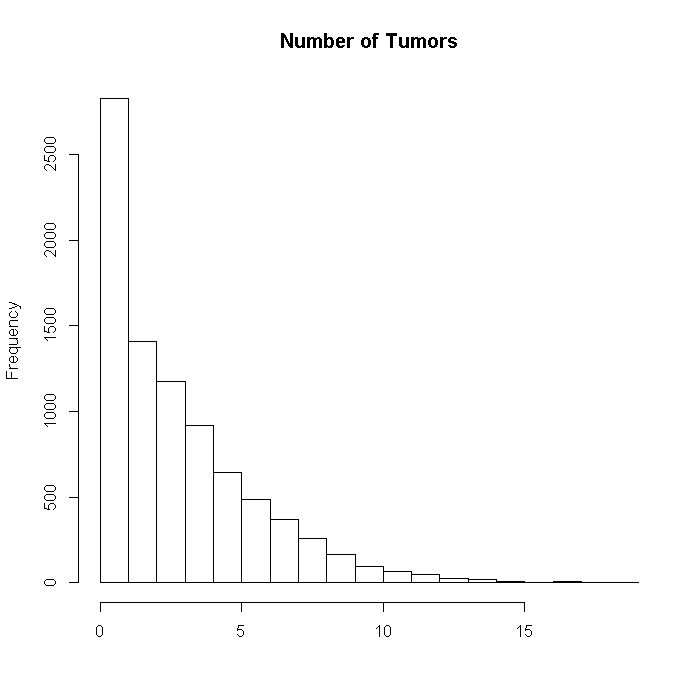
mntumor.true <- glmer(outcome$ntumors ~ Age + FamilyHx + LengthofStay +
  BMI + IL6 + CRP + SmokingHx + CancerStage +
  BMI:FamilyHx + Experience * CancerStage +
  (1 | DID) + (1 | HID), data = mldat, family = "poisson")

print(mntumor.true, correlation=FALSE)
## Generalized linear mixed model fit by the Laplace approximation
## Formula: outcome$ntumors ~ Age + FamilyHx + LengthofStay + BMI + IL6 +      CRP + SmokingHx + CancerStage + BMI:FamilyHx + Experience *      CancerStage + (1 | DID) + (1 | HID)
##    Data: mldat
##    AIC   BIC logLik deviance
##  11001 11135  -5482    10963
## Random effects:
##  Groups Name        Variance Std.Dev.
##  DID    (Intercept) 0.0297   0.172
##  HID    (Intercept) 0.1354   0.368
## Number of obs: 8525, groups: DID, 407; HID, 35
##
## Fixed effects:
##                            Estimate Std. Error z value Pr(>|z|)
## (Intercept)                0.192956   0.116514    1.66   0.0977 .
## Age                        0.008343   0.001180    7.07  1.5e-12 ***
## FamilyHxyes                0.241366   0.057603    4.19  2.8e-05 ***
## LengthofStay               0.000738   0.007321    0.10   0.9197
## BMI                        0.003400   0.001171    2.90   0.0037 **
## IL6                        0.005857   0.002131    2.75   0.0060 **
## CRP                        0.015431   0.001938    7.96  1.7e-15 ***
## SmokingHxformer           -0.108815   0.020177   -5.39  6.9e-08 ***
## SmokingHxnever            -0.252118   0.020727  -12.16  < 2e-16 ***
## CancerStageII              0.013703   0.075904    0.18   0.8567
## CancerStageIII             0.025328   0.084007    0.30   0.7630
## CancerStageIV              0.357715   0.088683    4.03  5.5e-05 ***
## Experience                -0.003144   0.004051   -0.78   0.4377
## FamilyHxyes:BMI            0.018063   0.001871    9.65  < 2e-16 ***
## CancerStageII:Experience   0.005583   0.004181    1.34   0.1818
## CancerStageIII:Experience  0.021037   0.004553    4.62  3.8e-06 ***
## CancerStageIV:Experience   0.030032   0.004785    6.28  3.5e-10 ***
## ---
## Signif. codes:  0 '***' 0.001 '**' 0.01 '*' 0.05 '.' 0.1 ' ' 1
Finally the outcome is censored at 9. We refit the same model, though now it is no longer exactly correct because it does not account for the censoring.
outcome$ntumors <- pmin(outcome$ntumors, 9)
hist(outcome$ntumors, xlab = "", main = "Number of Tumors")
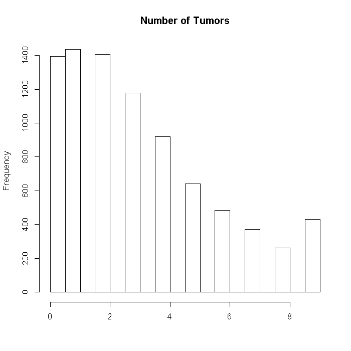
mntumor.true <- glmer(outcome$ntumors ~ Age + FamilyHx + LengthofStay +
    BMI + IL6 + CRP + SmokingHx + CancerStage + BMI:FamilyHx + Experience *
    CancerStage + (1 | DID) + (1 | HID), data = mldat, family = "poisson")

print(mntumor.true, correlation = FALSE)
## Generalized linear mixed model fit by the Laplace approximation
## Formula: outcome$ntumors ~ Age + FamilyHx + LengthofStay + BMI + IL6 +      CRP + SmokingHx + CancerStage + BMI:FamilyHx + Experience *      CancerStage + (1 | DID) + (1 | HID)
##    Data: mldat
##    AIC   BIC logLik deviance
##  10725 10859  -5343    10687
## Random effects:
##  Groups Name        Variance Std.Dev.
##  DID    (Intercept) 0.0276   0.166
##  HID    (Intercept) 0.1301   0.361
## Number of obs: 8525, groups: DID, 407; HID, 35
##
## Fixed effects:
##                           Estimate Std. Error z value Pr(>|z|)
## (Intercept)                0.23016    0.11582    1.99  0.04690 *
## Age                        0.00807    0.00119    6.76  1.3e-11 ***
## FamilyHxyes                0.32494    0.05892    5.51  3.5e-08 ***
## LengthofStay               0.00297    0.00741    0.40  0.68802
## BMI                        0.00334    0.00117    2.85  0.00439 **
## IL6                        0.00423    0.00217    1.95  0.05102 .
## CRP                        0.01521    0.00196    7.76  8.5e-15 ***
## SmokingHxformer           -0.11830    0.02036   -5.81  6.3e-09 ***
## SmokingHxnever            -0.26226    0.02092  -12.54  < 2e-16 ***
## CancerStageII              0.00278    0.07616    0.04  0.97085
## CancerStageIII             0.03325    0.08455    0.39  0.69410
## CancerStageIV              0.34549    0.09040    3.82  0.00013 ***
## Experience                -0.00397    0.00402   -0.99  0.32350
## FamilyHxyes:BMI            0.01356    0.00192    7.05  1.8e-12 ***
## CancerStageII:Experience   0.00657    0.00420    1.57  0.11727
## CancerStageIII:Experience  0.02049    0.00459    4.47  8.0e-06 ***
## CancerStageIV:Experience   0.02803    0.00489    5.74  9.6e-09 ***
## ---
## Signif. codes:  0 '***' 0.001 '**' 0.01 '*' 0.05 '.' 0.1 ' ' 1
Number of self-administered morphine doses
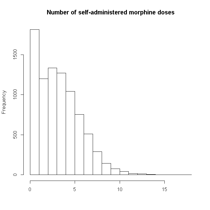
Now we will generate the data for the outcome, number of self-administered morphine doses. This actually has two components. Patients who had less severe disease had briefer surgeries and were not given morphine pumps. Thus all of these individuals had 0 doses. Whether or not (binary) a patient was given a morphine pump is based on cancer stage and number of tumors.
For patients who did have a morphine pump, the number of self-administered doses is drawn from a poisson distribution where the single parameter, lambda, is based on the vector of true coefficients premultiplied by the predictor matrix. Doctors (but not hospitals) have an effect for the number of doses administered (i.e., the poisson portion) but not for whether or not an individual was given a morphine pump (the zero inflation portion). Hospital (the third level) had no effect. The r(N, 2, .4, dat[, "BMI"])) specifies a random effect of BMI by doctor, where the coefficients are drawn from a normal distribution with mean 2 and standard deviation .4. From before, N is a vector whose length is the number of doctors and each element is the number of patients within each doctor. The final outcome is a zero-inflated poisson model.
set.seed(17828)
outcome$nmorphine <- pmin(
  rbinom(i, 1, logit(dat %*% b$zeroinflation + rnorm(i, mean = 8, sd = 4))) *
  rpois(n = i,
    pmax((dat %*% b$nmorphine + r(N, .6, .3, dat[, "BMI"]) + rnorm(i, mean = 22, sd = .1))/10, 0)),
  dat[, "LengthofStay"] * 4)
hist(outcome$nmorphine, xlab = "", main = "Number of self-administered morphine doses")
zeros <- as.numeric(outcome$nmorphine > 0)
mzero.true <- glmer(zeros ~ Age + SmokingHx + CancerStage +
  (1 | DID), data = mldat, family = "binomial")

print(mzero.true, correlation=FALSE)
## Generalized linear mixed model fit by the Laplace approximation
## Formula: zeros ~ Age + SmokingHx + CancerStage + (1 | DID)
##    Data: mldat
##   AIC  BIC logLik deviance
##  4389 4446  -2187     4373
## Random effects:
##  Groups Name        Variance Std.Dev.
##  DID    (Intercept) 4.56     2.14
## Number of obs: 8525, groups: DID, 407
##
## Fixed effects:
##                 Estimate Std. Error z value Pr(>|z|)
## (Intercept)      2.79721    0.39594    7.06  1.6e-12 ***
## Age              0.00985    0.00777    1.27      0.2
## SmokingHxformer -0.85873    0.14246   -6.03  1.7e-09 ***
## SmokingHxnever  -1.61570    0.13271  -12.17  < 2e-16 ***
## CancerStageII    1.07489    0.10446   10.29  < 2e-16 ***
## CancerStageIII   2.75482    0.16972   16.23  < 2e-16 ***
## CancerStageIV    3.42346    0.25283   13.54  < 2e-16 ***
## ---
## Signif. codes:  0 '***' 0.001 '**' 0.01 '*' 0.05 '.' 0.1 ' ' 1
mnmorphine.true <- glmer(outcome$nmorphine ~ Age + Sex + LengthofStay +
  CancerStage + (1 | DID) + (0 + BMI | DID), data = mldat, family = "poisson")

print(mnmorphine.true, correlation=FALSE)
## Generalized linear mixed model fit by the Laplace approximation
## Formula: outcome$nmorphine ~ Age + Sex + LengthofStay + CancerStage +      (1 | DID) + (0 + BMI | DID)
##    Data: mldat
##    AIC   BIC logLik deviance
##  12367 12431  -6175    12349
## Random effects:
##  Groups Name        Variance Std.Dev.
##  DID    (Intercept) 0.143670 0.3790
##  DID    BMI         0.000183 0.0135
## Number of obs: 8525, groups: DID, 407
##
## Fixed effects:
##                Estimate Std. Error z value Pr(>|z|)
## (Intercept)     1.04598    0.05879   17.79  < 2e-16 ***
## Age            -0.00172    0.00109   -1.57     0.12
## Sexmale        -0.06445    0.01204   -5.35  8.6e-08 ***
## LengthofStay    0.00560    0.00660    0.85     0.40
## CancerStageII   0.07849    0.01534    5.12  3.1e-07 ***
## CancerStageIII  0.20580    0.01852   11.11  < 2e-16 ***
## CancerStageIV   0.31352    0.02341   13.39  < 2e-16 ***
## ---
## Signif. codes:  0 '***' 0.001 '**' 0.01 '*' 0.05 '.' 0.1 ' ' 1
Cancer in remission
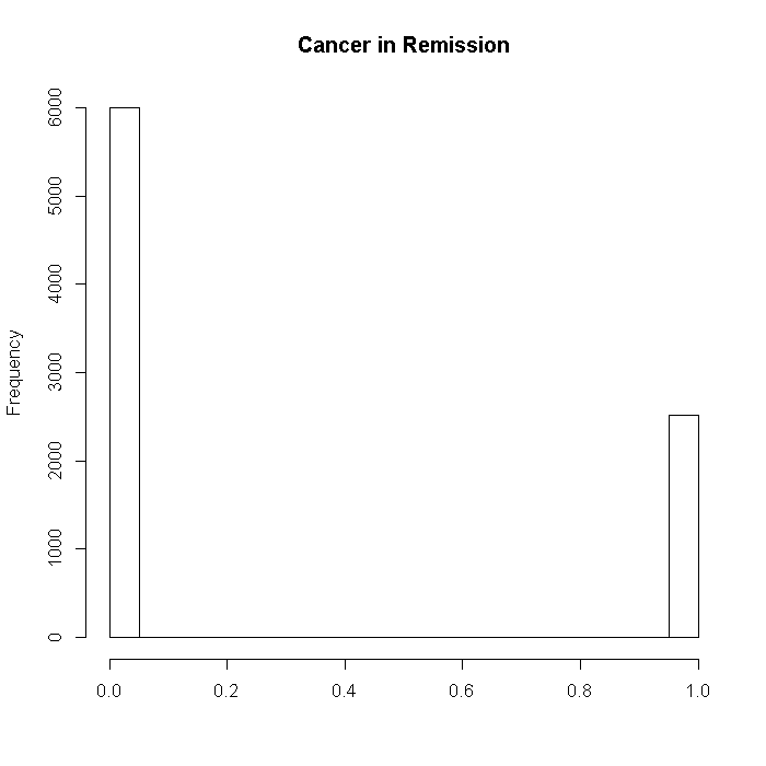
Now we can generate the data for the outcome, remission. First we create a vector of the true coefficients, which is premultiplied by the predictor matrix, and then the data will be drawn from a normal distribution with the expectation from our true model, and then cut at the upper quartile. The outcome is whether a patients cancer is in remission (TRUE or FALSE).
set.seed(41905)
tmp <- dat %*% b$remission + r(N, -1.5, 3, dat[, "LengthofStay"])
outcome$remission <- as.numeric(rnorm(n = i, mean = tmp, sd = 15) > quantile(tmp, probs = .75))
hist(outcome$remission, xlab = "", main = "Cancer in Remission")
mremission.true <- glmer(outcome$remission ~ Age + FamilyHx + LengthofStay +
  IL6 + CRP + CancerStage + Experience +
  (1 + LengthofStay | DID) + (1 | HID), data = mldat, family = "binomial")

print(mremission.true, correlation=FALSE)
## Generalized linear mixed model fit by the Laplace approximation
## Formula: outcome$remission ~ Age + FamilyHx + LengthofStay + IL6 + CRP +      CancerStage + Experience + (1 + LengthofStay | DID) + (1 |      HID)
##    Data: mldat
##   AIC  BIC logLik deviance
##  7148 7246  -3560     7120
## Random effects:
##  Groups Name         Variance Std.Dev. Corr
##  DID    (Intercept)  0.252    0.502
##         LengthofStay 0.152    0.390    -0.273
##  HID    (Intercept)  0.531    0.728
## Number of obs: 8525, groups: DID, 407; HID, 35
##
## Fixed effects:
##                Estimate Std. Error z value Pr(>|z|)
## (Intercept)     -0.5326     0.5307   -1.00  0.31559
## Age             -0.0154     0.0060   -2.57  0.01023 *
## FamilyHxyes     -1.3523     0.0961  -14.08  < 2e-16 ***
## LengthofStay    -0.1976     0.0420   -4.70  2.6e-06 ***
## IL6             -0.0592     0.0116   -5.09  3.5e-07 ***
## CRP             -0.0214     0.0103   -2.09  0.03697 *
## CancerStageII   -0.2968     0.0769   -3.86  0.00011 ***
## CancerStageIII  -0.8695     0.1025   -8.49  < 2e-16 ***
## CancerStageIV   -2.3089     0.1711  -13.50  < 2e-16 ***
## Experience       0.1061     0.0235    4.52  6.2e-06 ***
## ---
## Signif. codes:  0 '***' 0.001 '**' 0.01 '*' 0.05 '.' 0.1 ' ' 1
Proportion of optimal lung capacity
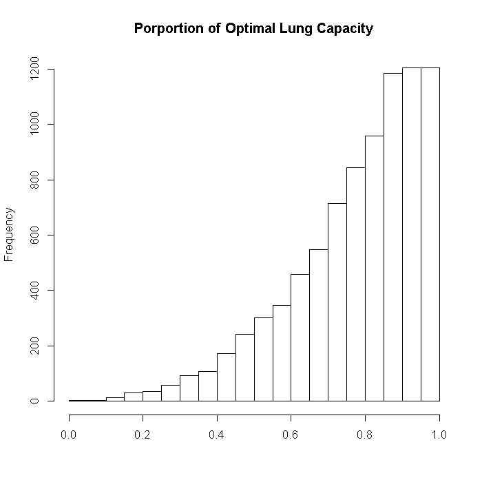
Now we can generate the data for the outcome, proportion of optimal lung capacity. The outcome is generated from a beta distribution where the first parameter is the exponentiated linear predictor, and the second is a constant at 1.2.
set.seed(10068)
outcome$lungcapacity <- rbeta(i, exp(pmin((dat %*% b$lungcapacity)/40 + 2, 2.5)), 1.2)
hist(outcome$lungcapacity, xlab = "", main = "Porportion of Optimal Lung Capacity")
Now we can check that we at least approximately recover our coefficients. Note that this is a very slow model to fit
## the beta family is not available in the lme4 package so load the
## glmmADMB package
require(glmmADMB)
mlungcapacity.true <- glmmadmb(outcome$lungcapacity ~ RBC + IL6:CRP +
    SmokingHx * FamilyHx + Experience + School + (1 | DID), data = mldat, family = "beta")

summary(mlungcapacity.true)
##
## Call:
## glmmadmb(formula = outcome$lungcapacity ~ RBC + IL6:CRP + SmokingHx *
##     FamilyHx + Experience + School + (1 | DID), data = mldat,
##     family = "beta")
##
##
## Coefficients:
##                              Estimate Std. Error z value Pr(>|z|)
## (Intercept)                  1.784036   0.180930    9.86  < 2e-16 ***
## RBC                         -0.140644   0.033174   -4.24  2.2e-05 ***
## SmokingHxformer             -0.063360   0.037271   -1.70    0.089 .
## SmokingHxnever              -0.025874   0.030935   -0.84    0.403
## FamilyHxyes                 -0.038940   0.043689   -0.89    0.373
## Experience                   0.007077   0.003633    1.95    0.051 .
## Schooltop                    0.021755   0.034380    0.63    0.527
## IL6:CRP                      0.004213   0.000476    8.85  < 2e-16 ***
## SmokingHxformer:FamilyHxyes  0.050211   0.066391    0.76    0.449
## SmokingHxnever:FamilyHxyes  -0.371804   0.057321   -6.49  8.8e-11 ***
## ---
## Signif. codes:  0 '***' 0.001 '**' 0.01 '*' 0.05 '.' 0.1 ' ' 1
##
## Number of observations: total=8525, DID=407
## Random effect variance(s):
## Group=DID
##             Variance StdDev
## (Intercept)  0.04468 0.2114
## Beta dispersion parameter: 5.26 (std. err.: 0.0804)
##
## Log-likelihood: 4689
Finally, we look at the structure of the final dataset and save it out as a CSV file.
finaldata <- cbind(outcome, mldat)
str(finaldata)
## 'data.frame':	8525 obs. of  27 variables:
##  $ tumorsize   : num  68 64.7 51.6 86.4 53.4 ...
##  $ co2         : num  1.53 1.68 1.53 1.45 1.57 ...
##  $ pain        : int  4 2 6 3 3 4 3 3 4 5 ...
##  $ wound       : int  4 3 3 3 4 5 4 3 4 4 ...
##  $ mobility    : int  2 2 2 2 2 2 2 3 3 3 ...
##  $ ntumors     : num  0 0 0 0 0 0 0 0 2 0 ...
##  $ nmorphine   : num  0 0 0 0 0 0 0 0 0 0 ...
##  $ remission   : num  0 0 0 0 0 0 0 0 0 0 ...
##  $ lungcapacity: num  0.801 0.326 0.565 0.848 0.886 ...
##  $ Age         : num  65 53.9 53.3 41.4 46.8 ...
##  $ Married     : num  0 0 1 0 0 1 1 0 1 0 ...
##  $ FamilyHx    : Factor w/ 2 levels "no","yes": 1 1 1 1 1 1 1 1 2 1 ...
##  $ SmokingHx   : Factor w/ 3 levels "current","former",..: 2 2 3 2 3 3 1 2 2 3 ...
##  $ Sex         : Factor w/ 2 levels "female","male": 2 1 1 2 2 2 1 2 2 2 ...
##  $ CancerStage : Factor w/ 4 levels "I","II","III",..: 2 2 2 1 2 1 2 2 2 2 ...
##  $ LengthofStay: num  6 6 5 5 6 5 4 5 6 7 ...
##  $ WBC         : num  6088 6700 6043 7163 6443 ...
##  $ RBC         : num  4.87 4.68 5.01 5.27 4.98 ...
##  $ BMI         : num  24.1 29.4 29.5 21.6 29.8 ...
##  $ IL6         : num  3.7 2.63 13.9 3.01 3.89 ...
##  $ CRP         : num  8.086 0.803 4.034 2.126 1.349 ...
##  $ DID         : Factor w/ 407 levels "1","2","3","4",..: 1 1 1 1 1 1 1 1 1 1 ...
##  $ Experience  : num  25 25 25 25 25 25 25 25 25 25 ...
##  $ School      : Factor w/ 2 levels "average","top": 1 1 1 1 1 1 1 1 1 1 ...
##  $ Lawsuits    : num  3 3 3 3 3 3 3 3 3 3 ...
##  $ HID         : Factor w/ 35 levels "1","2","3","4",..: 1 1 1 1 1 1 1 1 1 1 ...
##  $ Medicaid    : num  0.606 0.606 0.606 0.606 0.606 ...
## histogram matrix of all variables
hgraph(as.data.frame(lapply(finaldata, as.numeric)))
## save dataset
write.csv(finaldata, file = "z:/data/hdp.csv", row.names = FALSE,
    quote = FALSE)
