Version info: Code for this page was tested in R Under development (unstable) (2012-07-05 r59734)

 On: 2012-08-08

With: knitr 0.6.3
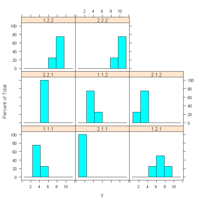
This code fragment covers a split-plot factorial design with one between subject factor and two within subject factors use the lmer command using a Stata dataset. In this dataset y is the response variable, a is the between subject factor, b and c are within subject factors, and s is the subject identifier. We also view a histogram for each plot to get a bit of a sense of the data.
library(foreign)  # to read the Stata file
library(lattice)  # for the graphics
library(lme4)  # to fit the model
spf <- read.dta("https://stats.idre.ucla.edu/stat/data/spf2-22.dta")

histogram(~y | interaction(a, b, c), data = spf)
m1 <- lmer(y ~ factor(a) * factor(b) * factor(c) + (1 | s), data = spf)

anova(m1)
## Analysis of Variance Table
##                               Df Sum Sq Mean Sq F value
## factor(a)                      1    1.0     1.0    2.00
## factor(b)                      1  162.0   162.0  319.56
## factor(c)                      1   24.5    24.5   48.33
## factor(a):factor(b)            1    6.1     6.1   12.08
## factor(a):factor(c)            1   10.1    10.1   19.97
## factor(b):factor(c)            1    8.0     8.0   15.78
## factor(a):factor(b):factor(c)  1    3.1     3.1    6.16