Version info: Code for this page was tested in R Under development (unstable) (2012-07-05 r59734)

 On: 2012-08-08

With: knitr 0.6.3
Singular value decomposition (SVD) is a type of matrix factorization.
For more details on SVD, the Wikipedia page
is a good starting point. On this page, we provide four examples of data
analysis using SVD in R.
Example 1: SVD to find a generalized inverse of a non-full-rank matrix
For a square matrix A with a non-zero determinant, there exists an inverse matrix B such that AB = I and
BA = I. For a matrix that is not square, generalized inverse matrices have
some (but not all) of the properties of an inverse matrix. SVD can be used to
find a generalized inverse matrix. In the example below, we use SVD to
find a generalized inverse B to the matrix A such that ABA = A. We compare our
generalized inverse with the one generated by the ginv command.
library(MASS)

a <- matrix(c(1, 1, 1, 1, 1, 1, 1, 1, 1, 1, 1, 1, 0, 0, 0, 0, 0,
    0, 0, 0, 0, 1, 1, 1, 0, 0, 0, 0, 0, 0, 0, 0, 0, 1, 1, 1), 9, 4)

a.svd <- svd(a)
a.svd$d
## [1] 3.46e+00 1.73e+00 1.73e+00 1.92e-16
ds <- diag(1/a.svd$d[1:3])
u <- a.svd$u
v <- a.svd$v
us <- as.matrix(u[, 1:3])
vs <- as.matrix(v[, 1:3])

(a.ginv <- vs %*% ds %*% t(us))
##         [,1]    [,2]    [,3]    [,4]    [,5]    [,6]    [,7]    [,8]
## [1,]  0.0833  0.0833  0.0833  0.0833  0.0833  0.0833  0.0833  0.0833
## [2,]  0.2500  0.2500  0.2500 -0.0833 -0.0833 -0.0833 -0.0833 -0.0833
## [3,] -0.0833 -0.0833 -0.0833  0.2500  0.2500  0.2500 -0.0833 -0.0833
## [4,] -0.0833 -0.0833 -0.0833 -0.0833 -0.0833 -0.0833  0.2500  0.2500
##         [,9]
## [1,]  0.0833
## [2,] -0.0833
## [3,] -0.0833
## [4,]  0.2500
# using the function ginv defined in MASS
ginv(a)
##         [,1]    [,2]    [,3]    [,4]    [,5]    [,6]    [,7]    [,8]
## [1,]  0.0833  0.0833  0.0833  0.0833  0.0833  0.0833  0.0833  0.0833
## [2,]  0.2500  0.2500  0.2500 -0.0833 -0.0833 -0.0833 -0.0833 -0.0833
## [3,] -0.0833 -0.0833 -0.0833  0.2500  0.2500  0.2500 -0.0833 -0.0833
## [4,] -0.0833 -0.0833 -0.0833 -0.0833 -0.0833 -0.0833  0.2500  0.2500
##         [,9]
## [1,]  0.0833
## [2,] -0.0833
## [3,] -0.0833
## [4,]  0.2500
Example 2: Image processing
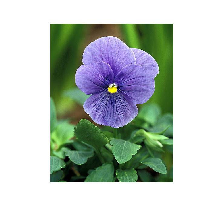
The code below requires the ReadImages package. It reads in a jpeg (pansy.jpg)
and plots it in R, first in color (when the image is stored as three
matrices–one red, one green, one blue) and then in grayscale (when the image is
stored as one matrix). Then, using SVD, we can essentially compress the image.
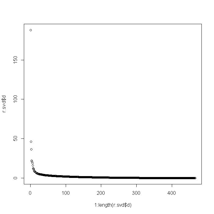
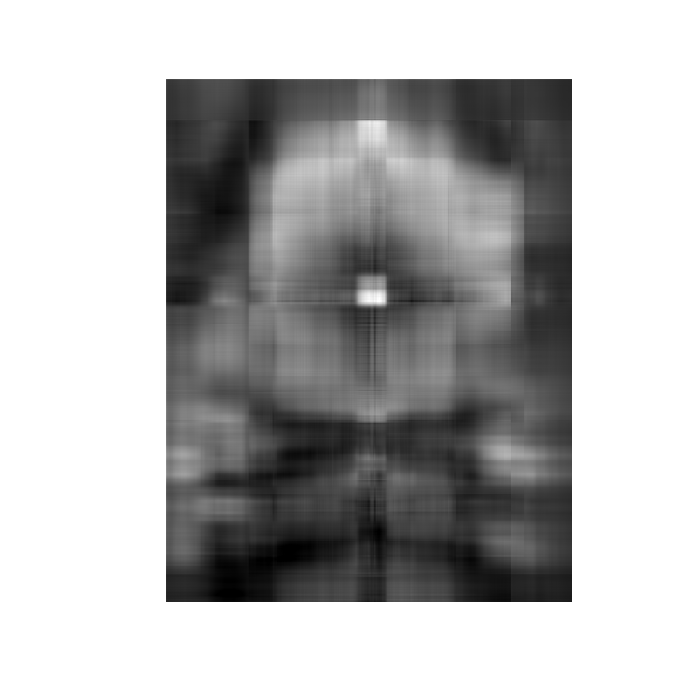
Note that we can recover the image to varying degrees of detail as we recreate
the image from different numbers of dimensions from our SVD matrices. You can
see how many dimensions are needed before you have an image that cannot be
differentiated from the original.

library(ReadImages)
x <- read.jpeg("pansy.jpg")
dim(x)
## [1] 600 465 3
plot(x, useRaster = TRUE)
r <- imagematrix(x, type = "grey")

plot(r, useRaster = TRUE)

r.svd <- svd(r)
d <- diag(r.svd$d)
dim(d)
## [1] 465 465
u <- r.svd$u
v <- r.svd$v
plot(1:length(r.svd$d), r.svd$d)
# first approximation
u1 <- as.matrix(u[-1, 1])
v1 <- as.matrix(v[-1, 1])
d1 <- as.matrix(d[1, 1])
l1 <- u1 %*% d1 %*% t(v1)
l1g <- imagematrix(l1, type = "grey")
plot(l1g, useRaster = TRUE)

# more approximation
depth <- 5
us <- as.matrix(u[, 1:depth])
vs <- as.matrix(v[, 1:depth])
ds <- as.matrix(d[1:depth, 1:depth])
ls <- us %*% ds %*% t(vs)
lsg <- imagematrix(ls, type = "grey")
## Warning: Pixel values were automatically clipped because of range over.
plot(lsg, useRaster = TRUE)
Example 3: Principal components analysis using SVD
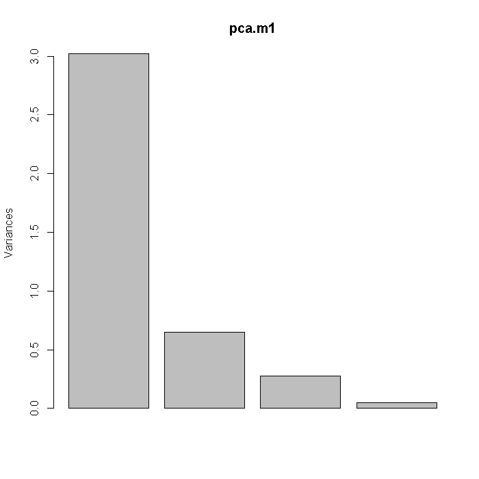
This example uses the Stata auto dataset. PCA can be achieved using SVD.
Below, we first use the prcomp command in R and then plot the variances
of the principal components (i.e. the square roots of the eigenvalues). These
values can also be found through spectral decomposition on the correlation
matrix or by SVD on the
variable matrix after standardizing each variable.
library(foreign)
auto <- read.dta("http://statistics.ats.ucla.edu/stat/data/auto.dta")

pca.m1 <- prcomp(~trunk + weight + length + headroom, data = auto,
    scale = TRUE)

screeplot(pca.m1)
# spectral decomposition: eigen values and eigen vectors
xvars <- with(auto, cbind(trunk, weight, length, headroom))
corr <- cor(xvars)
a <- eigen(corr)
(std <- sqrt(a$values))
## [1] 1.738 0.807 0.526 0.225
(rotation <- a$vectors)
##        [,1]   [,2]   [,3]    [,4]
## [1,] -0.507 -0.233  0.825  0.0921
## [2,] -0.522  0.454 -0.268  0.6708
## [3,] -0.536  0.390 -0.137 -0.7358
## [4,] -0.428 -0.767 -0.479 -0.0057
# svd approach
df <- nrow(xvars) - 1
zvars <- scale(xvars)
z.svd <- svd(zvars)
z.svd$d/sqrt(df)
## [1] 1.738 0.807 0.526 0.225
z.svd$v
##       [,1]   [,2]   [,3]    [,4]
## [1,] 0.507 -0.233  0.825 -0.0921
## [2,] 0.522  0.454 -0.268 -0.6708
## [3,] 0.536  0.390 -0.137  0.7358
## [4,] 0.428 -0.767 -0.479  0.0057
Example 4: Metric multi-dimensional scaling with SVD
This example uses the Stata cerealnut dataset.
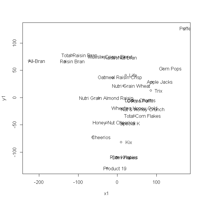
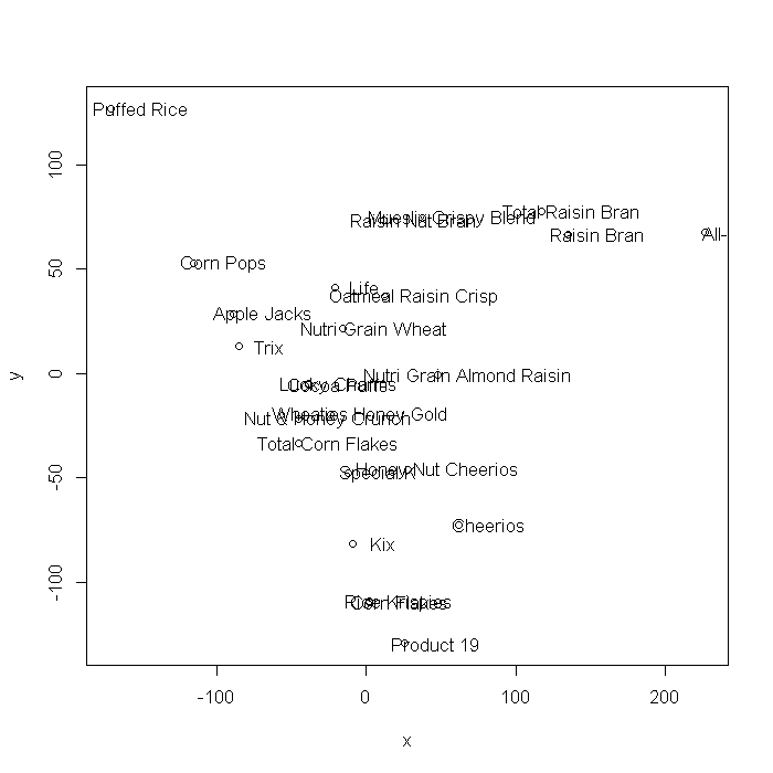
Multi-dimensional scaling can also be achieved using SVD. The plots generated
using cmdscale and the coordinates generated from the SVD steps are
mirrored about the x/x1 = 0 axis, but are otherwise identical.
cnut <- read.dta("http://statistics.ats.ucla.edu/stat/data/cerealnut.dta")

# centering the variables
mds.data <- as.matrix(sweep(cnut[, -1], 2, colMeans(cnut[, -1])))
dismat <- dist(mds.data)
mds.m1 <- cmdscale(dismat, k = 8, eig = TRUE)
mds.m1$eig
##  [1]  1.58e+05  1.09e+05  1.06e+04  3.83e+02  6.98e+01  1.25e+01  5.76e+00
##  [8]  2.22e+00  4.51e-12  4.51e-12  4.12e-12  3.19e-12  3.15e-12  2.30e-12
## [15]  2.09e-12  1.25e-12  1.13e-12  8.79e-13  2.97e-13 -1.38e-12 -1.45e-12
## [22] -1.57e-12 -1.88e-12 -5.92e-12 -2.52e-11
mds.m1 <- cmdscale(dismat, k = 2, eig = TRUE)
x <- mds.m1$points[, 1]
y <- mds.m1$points[, 2]
plot(x, y)
text(x + 20, y, label = cnut$brand)
# eigenvalues
xx <- svd(mds.data %*% t(mds.data))
xx$d
##  [1] 1.58e+05 1.09e+05 1.06e+04 3.83e+02 6.98e+01 1.25e+01 5.76e+00
##  [8] 2.22e+00 1.58e-11 9.90e-12 7.19e-12 4.71e-12 4.15e-12 3.03e-12
## [15] 2.77e-12 2.08e-12 1.97e-12 1.50e-12 1.26e-12 1.05e-12 7.93e-13
## [22] 7.35e-13 2.09e-13 1.65e-13 8.38e-14
# coordinates
xxd <- xx$v %*% sqrt(diag(xx$d))
x1 <- xxd[, 1]
y1 <- xxd[, 2]

plot(x1, y1)
text(x1 + 20, y1, label = cnut$brand)