Introduction
Power analysis is the name given to the process for determining the sample size for a research study. The technical definition of power is that it is the probability of detecting a “true” effect when it exists. Many students think that there is a simple formula for determining sample size for every research situation. However, the reality it that there are many research situations that are so complex that they almost defy rational power analysis. In most cases, power analysis involves a number of simplifying assumptions, in order to make the problem tractable, and running the analyses numerous times with different variations to cover all of the contingencies.
In this unit we will try to illustrate the power analysis process using a simple four group design.
Description of the Experiment
We wish to conduct a study in the area of mathematics education involving different teaching methods to improve standardized math scores in local classrooms. The study will include four different teaching methods and use fourth grade students who are randomly sampled from a large urban school district and are then random assigned to the four different teaching methods.
Here are the four different teaching methods which will be examined: 1) The traditional teaching method where the classroom teacher explains the concepts and assigns homework problems from the textbook; 2) the intensive practice method, in which students fill out additional work sheets both before and after school; 3) the computer assisted method, in which students learn math concepts and skills from using various computer based math learning programs; and, 4) the peer assistance learning method, which pairs each fourth grader with a fifth grader who helps them learn the concepts followed by the student teaching the same material to another student in their group.
Students will stay in their math learning groups for an entire academic year. At the end of the Spring semester all students will take the Multiple Math Proficiency Inventory (MMPI). This standardized test has a mean for fourth graders of 550 with a standard deviation of 80.
The experiment is designed so that each of the four groups will have the same sample size. One of the important questions we need to answer in designing the study is, how many students will be needed in each group?
The Power Analysis
In order to answer this question, we will need to make some assumptions and some educated guesses about the data. First, we will assume that the standard deviation for each of the four groups will be equal and will be equal to the national value of 80. Further, we expect, because of prior research, that the traditional teaching group (Group 1) will have the lowest mean score and that the peer assistance group (Group 4) will have the highest mean score on the MMPI. In fact, we expect that Group 1 will have a mean of 550 and that Group 4 will have mean that is greater by 1.2 standard deviations, i.e., the mean will equal at least 646. For the sake of simplicity, we will assume that the means of the other two groups will be equal to the grand mean.
We will make use power.anova.test in R to do the power analysis. This function needs the following information in order to do the power analysis: 1) the number of groups, 2) the between group variance 3) the within group variance, 4) the alpha level and 5) the sample size or power. As stated above, there are four groups, a=4. We will set alpha = 0.05. We already have the mean = 550 for the lowest group and the mean = 646 for the highest group. We will first set the means for the two middle groups to be the grand mean. Based on this setup and the assumption that the common standard deviation is equal to 80, we can do some simply calculation to see that the grand mean will be 598. Let’s first set the power to be .823 and calculate the corresponding sample size.
groupmeans <- c(550, 598, 598, 646)p <- power.anova.test(groups = length(groupmeans), between.var = var(groupmeans), within.var = 6400, power=0.823,sig.level=0.05,n=NULL) pBalanced one-way analysis of variance power calculation groups = 4 n = 16.98893 between.var = 1536 within.var = 6400 sig.level = 0.05 power = 0.823 NOTE: n is number in each group
Rounding 16.98 to 17, this means we need total of 17*4 = 68 subjects for a power of .823.
Now, if we want to see how sample size affects power, we can use a list of sample size and ask proc power to compute the power for us.
groupmeans <- c(550, 598, 598, 646)
n <- c(seq(2,10,by=1),seq(12,20,by=2),seq(25,50,by=5))
p <- power.anova.test(groups = length(groupmeans), between.var = var(groupmeans), within.var = 6400, power=NULL, sig.level=0.05,n=n) p Balanced one-way analysis of variance power calculation groups = 4 n = 2, 3, 4, 5, 6, 7, 8, 9, 10, 12, 14, 16, 18, 20, 25, 30, 35, 40, 45, 50 between.var = 1536 within.var = 6400 sig.level = 0.05 power = 0.09067458, 0.14381195, 0.20139579, 0.26146007, 0.32241923, 0.38293139, 0.44190044, 0.49846996, 0.55200591, 0.64840471, 0.72949120, 0.79552098, 0.84785780, 0.88840023, 0.95127832, 0.98006724, 0.99226927, 0.99713328, 0.99897699, 0.99964689 NOTE: n is number in each group
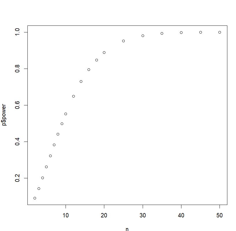
So we see that when we have 25 subjects in each group, we will have power of .95. We can also create a graph for the data above to visually inspect the relationship between sample size and power.
plot(n,p$power)
In the setup above, we have set it up so that the two middle groups will have means equal to the grand mean. Now in general, the means for the two middle groups can be anything in between. If you have a good idea on what these means should be, you might want to make use of this piece of information in your power analysis. For example, let’s say the means for the two middle groups should be 575 and 635. We will compute the power for a sequence of sample sizes as we did earlier.
groupmeans <- c(550, 575, 635, 646)
n <- c(seq(2,10,by=1),seq(12,20,by=2),seq(25,50,by=5))
p <- power.anova.test(groups = length(groupmeans),
between.var = var(groupmeans), within.var = 6400,
power=NULL, sig.level=0.05,n=n)
p
     Balanced one-way analysis of variance power calculation

groups = 4
n = 2, 3, 4, 5, 6, 7, 8,
9, 10, 12, 14, 16, 18, 20, 25,
30, 35, 40, 45, 50
between.var = 2152.333
within.var = 6400
sig.level = 0.05
power = 0.1079379, 0.1862722, 0.2707258,
0.3564714, 0.4400039, 0.5188111,
0.5912507, 0.6564086, 0.7139444,
0.8067917, 0.8734086, 0.9192133,
0.9496220, 0.9692210, 0.9916775,
0.9979422, 0.9995265, 0.9998974,
0.9999788, 0.9999958
So we see that for power of .8 we need fewer subjects than before when the two middle groups have the mean as the grand mean. This should be expected since the power here is the overall power of the F test for ANOVA and since the means are more polarized towards the two extreme ends, it is easier to detect the group effect.
Effect Size
The difference of the means between the lowest group and the highest group over the common standard deviation is a measure of effect size. In the calculation above, we have used 550 and 646 with common standard deviation of 80. This gives effect size of (646-550)/80 = 1.2. This is considered to be a large effect size. Let’s say now we have a medium effect size of .75. What does this translate into in terms of groups means? Well, we can always use 550 for the lowest group. The mean for the highest group will be .75*80 + 550 = 610. Let’s assume the two middle groups have the means of grand mean, say g. Then we have (550 + g + g + 610) / 4 = g. This gives us g = (550 + 610)/2 = 580. Let’s now redo our sample size calculation with this set of means.
groupmeans <- c(550,580,580,610)
p <- power.anova.test(groups = length(groupmeans),
between.var = var(groupmeans), within.var = 6400,
power=0.8, sig.level=0.05,n=NULL)
p

     Balanced one-way analysis of variance power calculation

         groups = 4
              n = 39.75519
    between.var = 600
     within.var = 6400
      sig.level = 0.05
          power = 0.8

NOTE: n is number in each group
So we see that at size of 40 (rounded up from 39.76) for each group, we have power of .8.
What about a small effect size, say, .25? We can do the same calculation as we did previously. The mean for each of the groups will be 550 , 560, 560, and 570.
groupmeans <- c(550,560,560,570)p <- power.anova.test(groups = length(groupmeans), between.var = var(groupmeans), within.var = 6400, power=0.8, sig.level=0.05,n=NULL) p Balanced one-way analysis of variance power calculation groups = 4 n = 349.8604 between.var = 66.66667 within.var = 6400 sig.level = 0.05 power = 0.8 NOTE: n is number in each group
Now the sample size goes way up (N=350).
Discussion
The sample size calculation is based a lot of assumptions. One of the assumptions for calculating the sample size for one-way ANOVA is the normality assumption for each group. We also assume that all the groups have the same common variance. Our power analysis calculation is based on these assumptions and we should be aware of it.
We have also assumed that we have knowledge of the magnitude of effect we are going to detect which is described in terms of group means in proc power. When we are unsure about the groups means, we should use more conservative estimates. For example, we might not have a good idea on the two means for the two middle group, then setting them to be the grand mean is more conservative than setting them to be something arbitrary.
Here are the sample sizes per group that we have come up with in our power analysis: 17 (best case scenario), 40 (medium effect size), and 350 (almost the worst case scenario). Even though we expect a large effect, we will shoot for a sample size of between 40 and 50. For one thing, it is all that our research budget will allow and the school district won’t allow us to use more than 200 students total.
References
Cohen, J. 1988. Statistical Power Analysis for the Behavioral Sciences, Second Edition. Mahwah, NJ: Lawrence Erlbaum Associates.