Truncated Regression

Truncated regression is used to model dependent variables for which some of the observations are not included in the analysis because of the value of the dependent variable.

This page uses the following packages. Make sure that you can load them before trying to run the examples on this page. If you do not have a package installed, run: install.packages("packagename"), or if you see the version is out of date, run: update.packages().

require(foreign)
require(ggplot2)
require(truncreg)
require(boot)

Version info: Code for this page was tested in R version 3.1.1 (2014-07-10) On: 2014-08-21 With: boot 1.3-11; truncreg 0.2-1; maxLik 1.2-0; miscTools 0.6-16; ggplot2 1.0.0; foreign 0.8-61; knitr 1.6

Please note: The purpose of this page is to show how to use various data analysis commands. It does not cover all aspects of the research process which researchers are expected to do. In particular, it does not cover data cleaning and checking, verification of assumptions, model diagnostics or potential follow-up analyses.

Examples of truncated regression

Example 1. A study of students in a special GATE (gifted and talented education) program wishes to model achievement as a function of language skills and the type of program in which the student is currently enrolled. A major concern is that students are required to have a minimum achievement score of 40 to enter the special program. Thus, the sample is truncated at an achievement score of 40.

Example 2. A researcher has data for a sample of Americans whose income is above the poverty line. Hence, the lower part of the distribution of income is truncated. If the researcher had a sample of Americans whose income was at or below the poverty line, then the upper part of the income distribution would be truncated. In other words, truncation is a result of sampling only part of the distribution of the outcome variable.

Description of the data

Let’s pursue Example 1 from above. We have a hypothetical data file, truncreg.dta, with 178 observations. The outcome variable is called achiv, and the language test score variable is called langscore. The variable prog is a categorical predictor variable with three levels indicating the type of program in which the students were enrolled.

Let’s look at the data. It is always a good idea to start with descriptive statistics.

dat <- read.dta("https://stats.idre.ucla.edu/stat/data/truncreg.dta")

summary(dat)

##        id            achiv        langscore          prog    
##  Min.   :  3.0   Min.   :41.0   Min.   :31.0   general : 40  
##  1st Qu.: 55.2   1st Qu.:47.0   1st Qu.:47.5   academic:101  
##  Median :102.5   Median :52.0   Median :56.0   vocation: 37  
##  Mean   :103.6   Mean   :54.2   Mean   :54.0                 
##  3rd Qu.:151.8   3rd Qu.:63.0   3rd Qu.:61.8                 
##  Max.   :200.0   Max.   :76.0   Max.   :67.0

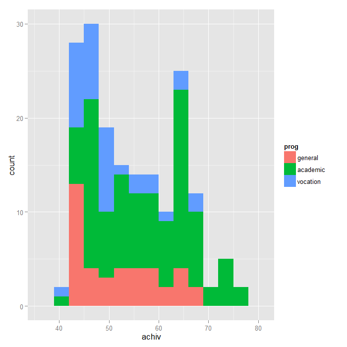
# histogram of achiv coloured by program type
ggplot(dat, aes(achiv, fill = prog)) +
  geom_histogram(binwidth=3)

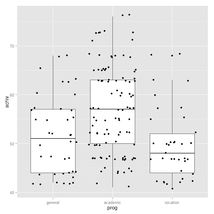
# boxplot of achiv by program type
ggplot(dat, aes(prog, achiv)) +
  geom_boxplot() +
  geom_jitter()

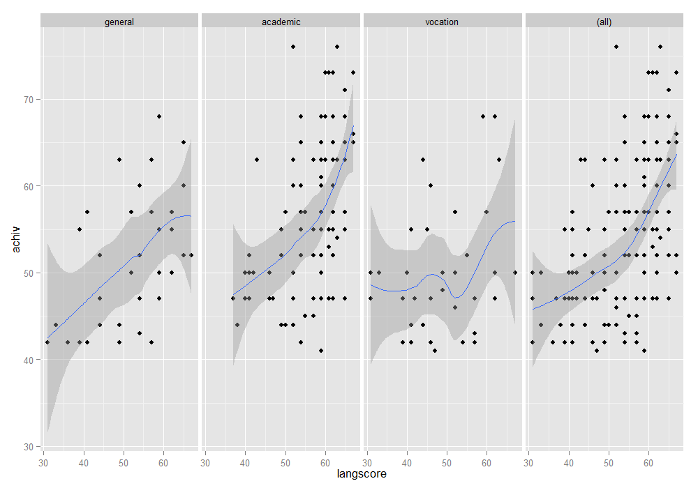
ggplot(dat, aes(x = langscore, y = achiv)) +
  geom_point() +
  stat_smooth(method = "loess") +
  facet_grid(. ~ prog, margins=TRUE)

Analysis methods you might consider

Below is a list of some analysis methods you may have encountered. Some of the methods listed are quite reasonable, while others have either fallen out of favor or have limitations.

OLS regression – You could analyze these data using OLS regression. OLS regression will not adjust the estimates of the coefficients to take into account the effect of truncating the sample at 40, and the coefficients may be severely biased. This can be conceptualized as a model specification error (Heckman, 1979).
Truncated regression – Truncated regression addresses the bias introduced when using OLS regression with truncated data. Note that with truncated regression, the variance of the outcome variable is reduced compared to the distribution that is not truncated. Also, if the lower part of the distribution is truncated, then the mean of the truncated variable will be greater than the mean from the untruncated variable; if the truncation is from above, the mean of the truncated variable will be less than the untruncated variable.
These types of models can also be conceptualized as Heckman selection models, which are used to correct for sampling selection bias.
Censored regression – Sometimes the concepts of truncation and censoring are confused. With censored data we have all of the observations, but we don’t know the “true” values of some of them. With truncation, some of the observations are not included in the analysis because of the value of the outcome variable. It would be inappropriate to analyze the data in our example using a censored regression model.

Below we use the truncreg function in the truncreg package to estimate a truncated regression model. The point argument indicates where the data are truncated, and the direction indicates whether it is left or right truncated.

m <- truncreg(achiv ~ langscore + prog, data = dat, point = 40, direction = "left")

summary(m)

## 
## Call:
## truncreg(formula = achiv ~ langscore + prog, data = dat, point = 40, 
##     direction = "left")
## 
## 
## Coefficients :
##              Estimate Std. Error t-value Pr(>|t|)    
## (Intercept)    11.299      6.772    1.67    0.095 .  
## langscore       0.713      0.114    6.23  4.8e-10 ***
## progacademic    4.063      2.054    1.98    0.048 *  
## progvocation   -1.144      2.670   -0.43    0.668    
## sigma           8.754      0.666   13.13  < 2e-16 ***
## ---
## Signif. codes:  0 '***' 0.001 '**' 0.01 '*' 0.05 '.' 0.1 ' ' 1
## 
## Log-Likelihood: -591 on 5 Df

In the table of coefficients, we have the truncated regression coefficients, the standard error of the coefficients, the Wald z-tests (coefficient/se), and the p-value associated with each z-test (shown as t-values).
The ancillary statistic /sigma is equivalent to the standard error of estimate in OLS regression. The value of 8.76 can be compared to the standard deviation of achievement which was 8.96. This shows a modest reduction. The output also contains an estimate of the standard error of sigma.
The variable langscore is statistically significant. A unit increase in language score leads to a .71 increase in predicted achievement. One of the indicator variables for prog is also statistically significant. Compared to general programs, academic programs are about 4.07 higher. To determine if prog itself is statistically significant, we can test models with it in and out for the two degree-of-freedom test of this variable.

# update old model dropping prog
m2 <- update(m, . ~ . - prog)

pchisq(-2 * (logLik(m2) - logLik(m)), df = 2, lower.tail = FALSE)

## 'log Lik.' 0.0252 (df=3)

The two degree-of-freedom chi-square test indicates that prog is a statistically significant predictor of achiv. We can get the expected means for each program at the mean of langscore by reparameterizing the model.

# create mean centered langscore to use later
dat <- within(dat, {mlangscore <- langscore - mean(langscore)})

malt <- truncreg(achiv ~ 0 + mlangscore + prog, data = dat, point = 40)
summary(malt)

## 
## Call:
## truncreg(formula = achiv ~ 0 + mlangscore + prog, data = dat, 
##     point = 40)
## 
## 
## Coefficients :
##              Estimate Std. Error t-value Pr(>|t|)    
## mlangscore      0.713      0.114    6.22  4.8e-10 ***
## proggeneral    49.789      1.897   26.24  < 2e-16 ***
## progacademic   53.853      1.150   46.82  < 2e-16 ***
## progvocation   48.653      2.140   22.73  < 2e-16 ***
## sigma           8.755      0.667   13.13  < 2e-16 ***
## ---
## Signif. codes:  0 '***' 0.001 '**' 0.01 '*' 0.05 '.' 0.1 ' ' 1
## 
## Log-Likelihood: -591 on 5 Df

Notice all that has changed is the intercept is gone and the program scores are now the expected values when langscore is at its mean for each type of program.

We could also calculate the bootstrapped confidence intervals if we wanted to. First, we define a function that returns the parameters of interest, and then use the boot function to run the bootstrap.

f <- function(data, i) {
  require(truncreg)
  m <- truncreg(formula = achiv ~ langscore + prog, data = data[i, ], point = 40)
  as.vector(t(summary(m)$coefficients[, 1:2]))
}

set.seed(10)

(res <- boot(dat, f, R = 1200, parallel = "snow", ncpus = 4))

## 
## ORDINARY NONPARAMETRIC BOOTSTRAP
## 
## 
## Call:
## boot(data = dat, statistic = f, R = 1200, parallel = "snow", 
##     ncpus = 4)
## 
## 
## Bootstrap Statistics :
##      original    bias    std. error
## t1*    11.299  0.303557      5.9327
## t2*     6.772 -0.055936      0.8620
## t3*     0.713 -0.004048      0.0965
## t4*     0.114 -0.000685      0.0137
## t5*     4.063 -0.053784      2.0333
## t6*     2.054 -0.001430      0.2411
## t7*    -1.144  0.021373      2.8721
## t8*     2.670  0.012132      0.2944
## t9*     8.754 -0.109523      0.5500
## t10*    0.666 -0.010924      0.0754

We could use the bootstrapped standard error to get a normal approximation for a significance test and confidence intervals for every parameter. However, instead we will get the percentile and bias adjusted 95 percent confidence intervals, using the boot.ci function.

# basic parameter estimates with percentile and bias adjusted CIs
parms <- t(sapply(c(1, 3, 5, 7, 9), function(i) {
    out <- boot.ci(res, index = c(i, i + 1), type = c("perc", "bca"))
    with(out, c(Est = t0, pLL = percent[4], pUL = percent[5], bcaLL = bca[4],
        bcaLL = bca[5]))
}))

# add row names
row.names(parms) <- names(coef(m))
# print results
parms

##                 Est    pLL    pUL   bcaLL  bcaLL
## (Intercept)  11.299 -1.258 22.297 -3.7231 21.320
## langscore     0.713  0.539  0.916  0.5508  0.944
## progacademic  4.063  0.058  8.011  0.0842  8.043
## progvocation -1.144 -6.805  4.277 -6.8436  4.250
## sigma         8.754  7.674  9.792  7.8896 10.110

The conclusions are the same as from the default model tests. You can compute a rough estimate of the degree of association for the overall model, by correlating achiv with the predicted value and squaring the result.

dat$yhat <- fitted(m)

# correlation
(r <- with(dat, cor(achiv, yhat)))

## [1] 0.552

# rough variance accounted for
r^2

## [1] 0.305

The calculated value of .31 is rough estimate of the R² you would find in an OLS regression. The squared correlation between the observed and predicted academic aptitude values is about 0.31, indicating that these predictors accounted for over 30% of the variability in the outcome variable.

Things to consider

The truncreg function is designed to work when the truncation is on the outcome variable in the model. It is possible to have samples that are truncated based on one or more predictors. For example, modeling college GPA as a function of high school GPA (HSGPA) and SAT scores involves a sample that is truncated based on the predictors, i.e., only students with higher HSGPA and SAT scores are admitted into the college.
You need to be careful about what value is used as the truncation value, because it affects the estimation of the coefficients and standard errors. In the example above, if we had used point = 39 instead of point = 40, the results would have been slightly different. It does not matter that there were no values of 40 in our sample.

References

Greene, W. H. (2003). Econometric Analysis, Fifth Edition. Upper Saddle River, NJ: Prentice Hall.
Heckman, J. J. (1979). Sample selection bias as a specification error. Econometrica, Volume 47, Number 1, pages 153 - 161.
Long, J. S. (1997). Regression Models for Categorical and Limited Dependent Variables. Thousand Oaks, CA: Sage Publications.