Applied Longitudinal Data Analysis: Modeling Change and Event Occurrence by Judith D. Singer and John B. Willett Chapter 12: Extending the Discrete-Time Hazard Model
The examples on the page were written in R version 2.4.1.
Table 12.2, page 413. To recreate this table, we will run each model separately and then combine the model statistics.
tenure <- read.table("https://stats.idre.ucla.edu/stat/examples/alda/tenure_pp.csv", sep=",", header=T)
attach(tenure)
PERIOD2 <- PERIOD^2
PERIOD3 <- PERIOD^3
PERIOD4 <- PERIOD^4
PERIOD5 <- PERIOD^5
PERIOD6 <- PERIOD^6
general <- glm(EVENT ~ D1 + D2 + D3 + D4 + D5 + D6 + D7 + D8 + D9, family = "binomial")
order0 <- glm(EVENT~1, family="binomial")
order1 <- glm(EVENT~PERIOD, family="binomial")
order2 <- glm(EVENT~PERIOD + PERIOD2, family="binomial")
order3 <- glm(EVENT~PERIOD + PERIOD2 + PERIOD3, family="binomial")
order4 <- glm(EVENT~PERIOD + PERIOD2 + PERIOD3 + PERIOD4, family="binomial")
order5 <- glm(EVENT~PERIOD + PERIOD2 + PERIOD3 + PERIOD4 + PERIOD5, family="binomial")
dev <- c(order0$deviance, order1$deviance, order2$deviance, order3$deviance, order4$deviance, order5$deviance, general$deviance)
dev.diff.p <- c(0, dev[1:5] - dev[2:6])
dev.diff.gen <- c(dev - dev[7])
aic <- c(order0$aic, order1$aic, order2$aic, order3$aic, order4$aic, order5$aic, general$aic)
table12.2 <- cbind(dev, dev.diff.p, dev.diff.gen, aic)
table12.2


           dev   dev.diff.p dev.diff.gen       aic
[1,] 1037.5652   0.00000000   206.361395 1039.5652
[2,]  867.4619 170.10332478    36.258070  871.4619
[3,]  836.3041  31.15779577     5.100274  842.3041
[4,]  833.1725   3.13158698     1.968687  841.1725
[5,]  832.7427   0.42981046     1.538877  842.7427
[6,]  832.7322   0.01051811     1.528358  844.7322
[7,]  831.2038   0.00000000     0.000000  849.2038
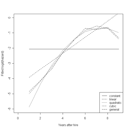
Figure 12.1, page 414. First, we will rerun the general model without an intercept for greater ease in using the model coefficients later.
general <- glm(EVENT ~ D1 + D2 + D3 + D4 + D5 + D6 + D7 + D8 + D9 - 1, family = "binomial")
In the loop below, we will use our model estimates to generate a fitted value for each of the nine time points from each of the models. These are the values that will be plotted in the first of the three plots. We also calculate the survival and hazard rates from the quadratic and general models to be plotted in the second and third graphs.
fits  <- c()
survivor.quad = 1
survivor.gen = 1
for (i in 1:9){
  constant = order0$coef[1]
  linear = order1$coef[1] + order1$coef[2]*i
  quadratic = order2$coef[1] + order2$coef[2]*i + order2$coef[3]*i**2
  cubic = order3$coef[1] + order3$coef[2]*i + order3$coef[3]*i**2 + order3$coef[4]*i**3
  hazard.quad = 1/(1 + exp(-quadratic));
  survivor.quad = (1 - hazard.quad)*survivor.quad;
  generalval = general$coef[i]
  hazard.gen = 1/(1 + exp(-generalval));
  survivor.gen = (1 - hazard.gen)*survivor.gen;
  z <- c(i, constant, linear, quadratic, cubic, generalval, hazard.quad, survivor.quad, hazard.gen, survivor.gen)
  fits <- rbind(fits, z)}
Each of the three graphs is created by generating the plot area while plotting one line, and then overlaying any additional lines on the same plot.
par(mfrow=c(1,1))
plot(fits[,1], fits[,2], type = "l", lty = 1, xlim = c(0,9), ylim = c(-6,0), xlab = "Years after hire", ylab = "Fitted logit(hazard)")
points(fits[,1], fits[,3], type = "l", lty = 2)
points(fits[,1], fits[,4], type = "l", lty = 3)
points(fits[,1], fits[,5], type = "l", lty = 4)
points(fits[,1], fits[,6], type = "l", lty = 5)
legend("bottomright", c("constant", "linear", "quadratic", "cubic", "general"), lty = c(1, 2, 3, 4, 5))
 par(mfrow=c(1,2))
plot(fits[,1], fits[,7], type = "l", lty = 1, xlim = c(0,9), ylim = c(0,.4), xlab = "Years after hire", ylab = "Fitted hazard")
points(fits[,1], fits[,9], type = "l", lty = 2)
legend("bottomright", c("quadratic","general"), lty = c(1, 2))
plot(fits[,1], fits[,8], type = "l", lty = 1, xlim = c(0,9), ylim = c(0,1), xlab = "Years after hire", ylab = "Fitted survival")
points(fits[,1], fits[,10], type = "l", lty = 2)
legend("bottomleft", c("quadratic","general"), lty = c(1, 2))
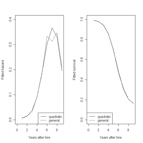
Figure 12.3, page 423. After reading in the data, we will subset it by parenting transition (PT) values. Then, we will run separate models on these datasets using both logit and cloglog transformations–four models in total. Finally, we will plot the parameter estimates associated with each of the time points from each of the four models.
firstsex<-read.table("https://stats.idre.ucla.edu/stat/examples/alda/firstsex_pp.csv", sep=",", header=T)
firstsex0  <- subset(firstsex, pt==0)
firstsex1  <- subset(firstsex, pt==1)
fs0.logit<-glm(event~d7+d8+d9+d10+d11+d12 - 1, family=binomial(link = "logit"), data = firstsex0)
fs1.logit<-glm(event~d7+d8+d9+d10+d11+d12 - 1, family=binomial(link = "logit"), data = firstsex1)
fs0.loglog<-glm(event~d7+d8+d9+d10+d11+d12 - 1, family=binomial(link = "cloglog"), data = firstsex0)
fs1.loglog<-glm(event~d7+d8+d9+d10+d11+d12 - 1, family=binomial(link = "cloglog"), data = firstsex1)
Having run these four models, we create a single dataset that contains the coefficients from each model and a column of time points. This is the dataset we will use to generate the plot. First, we create a plot with one of the lines. Then, we overlay the other three lines.
fig12.3 <- cbind(time = c(7, 8, 9 , 10, 11, 12), fs0.logit = fs0.logit$coef, fs0.loglog = fs0.loglog$coef, fs1.logit = fs1.logit$coef, fs1.loglog = fs1.loglog$coef)
par(mfrow=c(1,1))
plot(fig12.3[,1], fig12.3[,2], type = "l", ylab = "Transformed hazard probability", xlab = "Grade", ylim = c(-4,0))
points(fig12.3[,1], fig12.3[,3], type = "l", lty=2)
points(fig12.3[,1], fig12.3[,4], type = "l", lty=3)
points(fig12.3[,1], fig12.3[,5], type = "l", lty=4)
legend(7, 0, c("pt=0, logit", "pt=0, loglog", "pt=1, logit", "pt=1, loglog"), lty = c(1, 2, 3, 4))
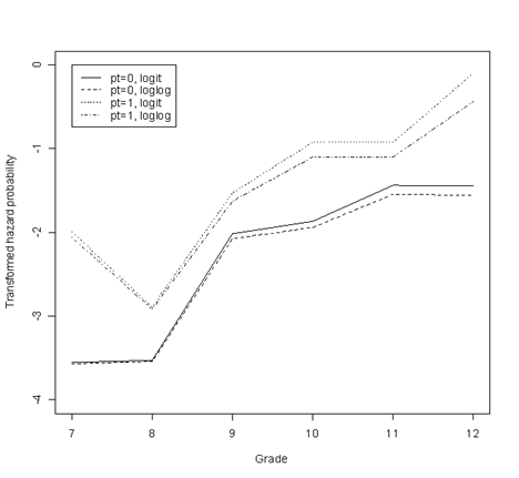
Table 12.3, page 424. For this table, we will run two models with different link functions and then find the fitted baseline hazard using the corresponding model coefficients.
fs.loglog<-glm(event~d7+d8+d9+d10+d11+d12+pt - 1, family=binomial(link = "cloglog"), data = firstsex)
fs.logit<-glm(event~d7+d8+d9+d10+d11+d12+pt - 1, family=binomial(link = "logit"), data = firstsex)

est.logit <- fs.logit$coef
est.loglog <- fs.loglog$coef
fbh.logit <- 1/(1+exp(-est.logit))
fbh.loglog <- 1-exp(-exp(est.loglog))

tab12.3 <- cbind(est.loglog, est.logit, fbh.loglog, fbh.logit)
tab12.3

    est.loglog  est.logit fbh.loglog  fbh.logit
d7  -2.9732973 -2.9943266 0.04984906 0.04768284
d8  -3.6592441 -3.7001239 0.02542322 0.02412410
d9  -2.3156320 -2.2811235 0.09398896 0.09269841
d10 -1.9001387 -1.8225985 0.13890279 0.13912236
d11 -1.7621385 -1.6542272 0.15774911 0.16053845
d12 -1.3426380 -1.1790570 0.22983911 0.23522180
pt   0.7854048  0.8736184 0.88845136 0.70549806

fs.loglog$deviance
[1] 634.5013

fs.logit$deviance
[1] 634.6618
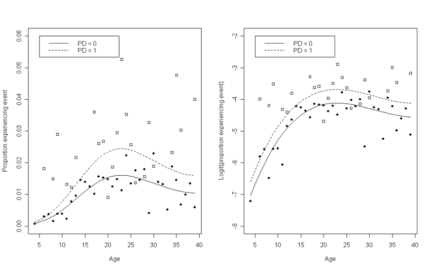
Figure 12.4, page 432. To generate these graphs, we will first do the calculations required for the scatter plots. Then we will run the model required to add the curves.
depression<-read.table("https://stats.idre.ucla.edu/stat/examples/alda/depression_pp.csv", sep=",", header=T)
For each age between 4 and 39, we are interested in the proportion of subjects that experienced the event (in this example, an initial depressive episode) within the group of subjects with divorced parents (PD = 1) and the group of subjects without divorced parents (PD = 0). To calculate this, we can loop through these combinations of age and PD values, subsetting our data and calculating the proportion within each subset. For the second graph, we will take the logit of this proportion.
percents <- c()
for (i in 4:39){
  for (j in 0:1){
    x <- subset(depression, PERIOD==i & PD==j)
    y <- table(x$EVENT)
    if (dim(y)==2){
      z <- c(i, j, y[[2]], y[[1]], (y[[2]]/(y[[1]]+y[[2]])))}
    if (dim(y)==1){
      z <- c(i, j, 0, y[[1]], NA)}
    percents <- rbind(percents, z)
  }
}

percents <- cbind(percents, log(percents[,5]/(1-percents[,5])))
colnames(percents) <- c("age", "parent", "event", "nonevent", "percent", "logpercent")
percents.nm <- as.data.frame(na.omit(percents))
percent.pd0 <- subset(percents.nm, parent == 0)
percent.pd1 <- subset(percents.nm, parent == 1)
Next, we will fit a logistic model to the data. Then, for each age between 4 and 39 and for each PD group, we are interested in the model-predicted proportion of subjects that experienced the event. To calculate this, we can again loop through these combinations of age and PD values and use the model coefficients to generate predicted proportions. We can also calculate the hazard rate for the second plot.
dmodel<-glm(EVENT ~ ONE + age_18 + age_18sq + age_18cub + PD - 1, family=binomial(link = "logit"), data = depression)

modelfit<- c()
for (i in 0:1){
  for (j in 4:39){
    fitx = dmodel$coef[1] + dmodel$coef[2]*(j-18) + dmodel$coef[3]*(j-18)^2 + dmodel$coef[4]*(j-18)^3 + dmodel$coef[5]*i
    fithazard = 1/(1 + exp(-fitx))
    modelfit <- rbind(modelfit, c(i, j, fitx, fithazard))
  }
}
Lastly, we subset our data and generate the plots, starting each with one scatter plot, then layering on the other scatter points and the two fitted curves.
modelfit.0 <- subset(data.frame(modelfit), modelfit[,1]==0)
modelfit.1 <- subset(data.frame(modelfit), modelfit[,1]==1)

par(mfrow=c(1,2))
plot(percent.pd0$age, percent.pd0$percent, pch = 19, ylim = c(0, .06), xlab = "Age", ylab = "Proportion experiencing event")
points(percent.pd1$age, percent.pd1$percent, pch = 22)
points(modelfit.0[,2], modelfit.0[,4], type = 'l', lty = 1)
points(modelfit.1[,2], modelfit.1[,4], type = 'l', lty = 2)
legend(5, 0.06, c("PD = 0", "PD = 1"), lty = c(1, 2))

plot(percent.pd0$age, percent.pd0$logpercent, pch = 19, ylim = c(-8, -2), xlab = "Age", ylab = "Logit(proportion experiencing event)")
points(percent.pd1$age, percent.pd1$logpercent, pch = 22)
points(modelfit.0[,2], modelfit.0[,3], type = 'l', lty = 1)
points(modelfit.1[,2], modelfit.1[,3], type = 'l', lty = 2)
legend(5, -2, c("PD = 0", "PD = 1"), lty = c(1, 2))
Figure 12.5, page 437. To generate these graphs, we will first fit a logistic regression model that predicts the event using three age terms, parental divorce, and sex.
depression<-read.table("https://stats.idre.ucla.edu/stat/examples/alda/depression_pp.csv", sep=",", header=T)

dmodel<-glm(EVENT ~ ONE + age_18 + age_18sq + age_18cub + PD + FEMALE - 1, family=binomial(link = "logit"), data = depression)
Next, we can to use the model coefficients to generate predicted values for all of the time/PD/sex combinations we are interested in. We will do this in a loop. Within each PD/sex combination, we are also interested in the “survival” rate at each time point. This will be the proportion of subjects that have not yet experienced the event at a given time point. Both the hazard and the survival rate will be calculated in the loop using the predicted values from the model. We will then subset the data by PD/sex combination, resulting in four datasets with one observation for each time point.
modelfit<- c()
for (i in 0:1){
  for (k in 0:1){
  survivor <- 1
    for (j in 4:39){
    fitx = dmodel$coef[1] + dmodel$coef[2]*(j-18) + dmodel$coef[3]*(j-18)^2 + dmodel$coef[4]*(j-18)^3 + dmodel$coef[5]*i + dmodel$coef[6]*k
    hazard = 1/(1 + exp(-fitx))
    survivor = (1-hazard)*survivor
    modelfit <- rbind(modelfit, c(i, j, k, fitx, hazard, survivor))}}}

colnames(modelfit) <- c("pd", "age", "female", "fit", "hazard", "survival")

modelfit.0male <- subset(data.frame(modelfit), modelfit[,1]==0 & modelfit[,3]==0)
modelfit.0female <- subset(data.frame(modelfit), modelfit[,1]==0 & modelfit[,3]==1)
modelfit.1male <- subset(data.frame(modelfit), modelfit[,1]==1 & modelfit[,3]==0)
modelfit.1female <- subset(data.frame(modelfit), modelfit[,1]==1 & modelfit[,3]==1)
To plot the four curves in each plot, we start with one plot, and then overlay the other three lines in the same plot area.
par(mfrow=c(1,2))

plot(modelfit.0male$age, modelfit.0male$hazard, type = 'l', lty = 1, ylim = c(0, .04), xlab = "Age", ylab = "Fitted hazard")
points(modelfit.0female$age, modelfit.0female$hazard, type = 'l', lty = 2)
points(modelfit.1male$age, modelfit.1male$hazard, type = 'l', lty = 3)
points(modelfit.1female$age, modelfit.1female$hazard, type = 'l', lty = 4)
legend(5, 0.04, c("PD = 0, Male", "PD = 0, Female", "PD = 1, Male", "PD = 1, Female"), lty = c(1, 2, 3, 4))


plot(modelfit.0male$age, modelfit.0male$survival, type = 'l', lty = 1, ylim = c(0, 1), xlab = "Age", ylab = "Fitted survival")
points(modelfit.0female$age, modelfit.0female$survival, type = 'l', lty = 2)
points(modelfit.1male$age, modelfit.1male$survival, type = 'l', lty = 3)
points(modelfit.1female$age, modelfit.1female$survival, type = 'l', lty = 4)
legend(0, 0.2, c("PD = 0, Male", "PD = 0, Female", "PD = 1, Male", "PD = 1, Female"), lty = c(1, 2, 3, 4))
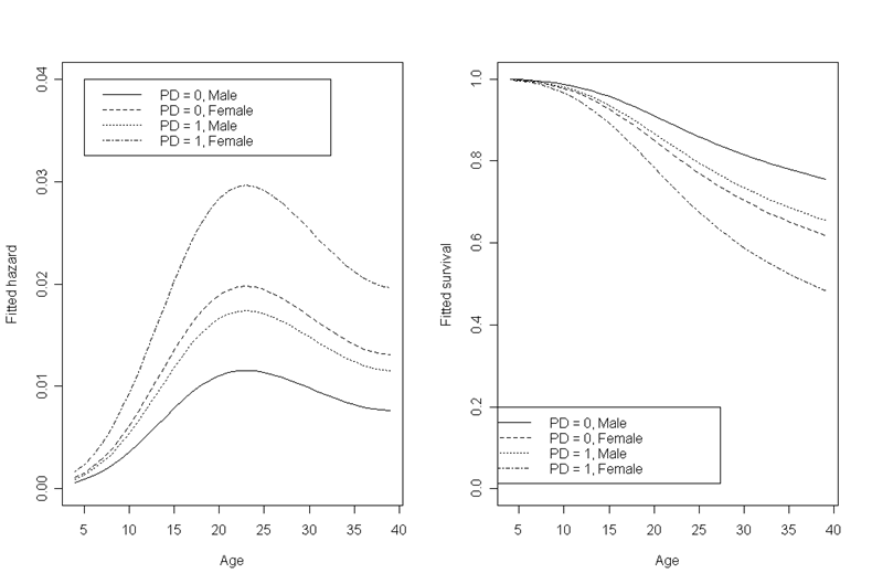
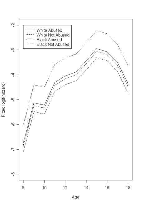
Figure 12.6, page 445. This set of plots is similar to previous examples: we will first calculate the proportion of a subset of subjects who experienced the event at a each time point, and then create plots of the proportion (or some transformation) against time with different lines representing different subject characteristics.
fa<-read.table("https://stats.idre.ucla.edu/stat/examples/alda/firstarrest_pp.csv", sep=",", header=T)
We loop through all of the combinations of time, race, and abused status in our dataset, subsetting on each and calculating the proportion of subjects experiencing the event within each subset. We then take the logit of this proportion. After completing the loop, we subset the percent and logit data into four datasets, one for each race/abuse combination.
percents <- c()
for (i in 8:18){
  for (j in 0:1){
    for (k in 0:1){
      x <- subset(fa, PERIOD==i & BLACK==j & ABUSED==k)
      if (sum(x$EVENT) > 0){
        y <- mean(x$EVENT)}
      if (sum(x$EVENT)==0){
        y <- NA}
      logity <- log(y/(1-y))
      z <- c(i, j, k, y, logity)
      percents <- rbind(percents, z)}}}

colnames(percents) <- c("age", "black", "abused", "pct", "hazard")
percents.nm <- as.data.frame(na.omit(percents))

percents.w.a <- subset(percents.nm, black==0 & abused==1)
percents.b.a <- subset(percents.nm, black==1 & abused==1)
percents.w.na <- subset(percents.nm, black==0 & abused==0)
percents.b.na <- subset(percents.nm, black==1 & abused==0)
Next, we create two plots: one of the white subjects and one of the black subjects. In each, we first plot a line for one of the abuse categories, and then overlay a line for the other.
par(mfrow=c(1,2))
plot(percents.w.a$age, percents.w.a$hazard, type = "l", lty = 1, ylim = c(-7, -2), xlim = c(8,18),
main = "White", xlab = "Age", ylab = "Sample logit(hazard)")
points(percents.w.na$age, percents.w.na$hazard, type = "l", lty = 2)
legend(8, -2, c("Abused", "Not Abused"), lty = c(1, 2))

plot(percents.b.a$age, percents.b.a$hazard, type = "l", lty = 1, ylim = c(-7, -2), xlim = c(8,18),
main = "Black", xlab = "Age", ylab = "Sample logit(hazard)")
points(percents.b.na$age, percents.b.na$hazard, type = "l", lty = 2)
legend(8, -2, c("Abused", "Not Abused"), lty = c(1, 2))
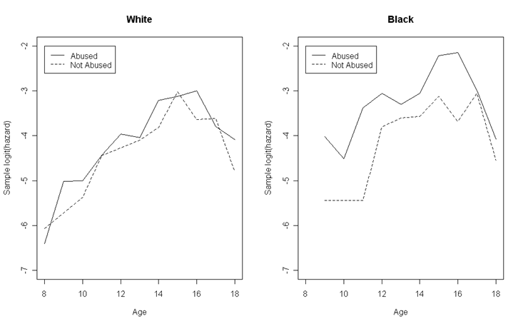
The first two graphs were created using raw proportions. The third graph is based on a logistic model fitted to the data, using time, race, abuse status, and an abuse-race interaction term as predictors. We will run this model and then use the coefficients to predict hazard rates at each time point for each race/abuse combination. These predicted values will be generated using a loop, as we have done in previous examples.
famodel<-glm(EVENT ~ D8 + D9 + D10 + D11 + D12 + D13 + D14 + D15 + D16 + D17 + D18 + ABUSED + BLACK + ABLACK - 1,
family=binomial(link = "logit"), data = fa)

modelfit <- c()
for (j in 0:1){
  for (k in 0:1){
  survivor <- 1
    for (i in 8:18){
      logitfit <- famodel$coef[i-7] + famodel$coef[12]*j + famodel$coef[13]*k + famodel$coef[14]*j*k
      hazard = 1/(1 + exp(-logitfit))
      survivor = (1-hazard)*survivor
      z <- c(i, j, k, j*k, logitfit, hazard, survivor)
      modelfit <- rbind(modelfit, z)}}}
After completing the loop, we will subset our data as we did for the first two plots. Then, we create one graph by plotting the line for one of the four race/abuse combinations and then overlaying the other three lines.
colnames(modelfit) <- c("age", "abused", "black", "ablack", "logitfit", "hazard", "survival")
modelfit <- as.data.frame(modelfit)
modelfit.w.a <- subset(modelfit, black==0 & abused==1)
modelfit.b.a <- subset(modelfit, black==1 & abused==1)
modelfit.w.na <- subset(modelfit, black==0 & abused==0)
modelfit.b.na <- subset(modelfit, black==1 & abused==0)

par(mfrow=c(1,1))
plot(modelfit.w.a$age, modelfit.w.a$logitfit, type = "l", lty = 1, ylim = c(-8, -2), xlim = c(8,18), xlab = "Age", ylab = "Fitted logit(hazard)")
points(modelfit.w.na$age, modelfit.w.na$logitfit, type = "l", lty = 2)
points(modelfit.b.a$age, modelfit.b.a$logitfit, type = "l", lty = 3)
points(modelfit.b.na$age, modelfit.b.na$logitfit, type = "l", lty = 4)
legend(8, -2, c("White Abused", "White Not Abused", "Black Abused", "Black Not Abused"), lty = c(1, 2, 3, 4))
Table 12.4, page 449. The parameter estimates and fit statistics in this table can be found in the output from each of the three models below.
depression<-read.table("https://stats.idre.ucla.edu/stat/examples/alda/depression_pp.csv", sep=",", header=T)

modelA<-glm(EVENT ~ ONE + age_18 + age_18sq + age_18cub + PD + FEMALE + NSIBS- 1,
  family=binomial(link = "logit"), data = depression)
summary(modelA)

Coefficients:
            Estimate Std. Error z value Pr(>|z|)
ONE       -4.359e+00  1.216e-01 -35.845  < 2e-16 ***
age_18     6.106e-02  1.166e-02   5.236 1.64e-07 ***
age_18sq  -7.308e-03  1.224e-03  -5.972 2.34e-09 ***
age_18cub  1.816e-04  7.897e-05   2.300 0.021447 *
PD         3.726e-01  1.624e-01   2.295 0.021754 *
FEMALE     5.587e-01  1.095e-01   5.103 3.34e-07 ***
NSIBS     -8.141e-02  2.227e-02  -3.655 0.000257 ***
---
Signif. codes:  0 '***' 0.001 '**' 0.01 '*' 0.05 '.' 0.1 ' ' 1

(Dispersion parameter for binomial family taken to be 1)

    Null deviance: 51288.7  on 36997  degrees of freedom
Residual deviance:  4124.3  on 36990  degrees of freedom
AIC: 4138.3

modelB<-glm(EVENT ~ ONE + age_18 + age_18sq + age_18cub + PD + FEMALE + SIBS12 + SIBS34 + SIBS56 + SIBS78 + SIBS9PLUS - 1,
  family=binomial(link = "logit"), data = depression)
summary(modelB)

Coefficients:
            Estimate Std. Error z value Pr(>|z|)
ONE       -4.500e+00  2.067e-01 -21.773  < 2e-16 ***
age_18     6.145e-02  1.166e-02   5.269 1.37e-07 ***
age_18sq  -7.289e-03  1.224e-03  -5.958 2.56e-09 ***
age_18cub  1.813e-04  7.897e-05   2.296   0.0217 *
PD         3.727e-01  1.625e-01   2.294   0.0218 *
FEMALE     5.596e-01  1.095e-01   5.109 3.24e-07 ***
SIBS12     2.085e-02  1.976e-01   0.106   0.9160
SIBS34     1.076e-02  2.100e-01   0.051   0.9591
SIBS56    -4.942e-01  2.545e-01  -1.942   0.0522 .
SIBS78    -7.754e-01  3.437e-01  -2.256   0.0241 *
SIBS9PLUS -6.585e-01  3.440e-01  -1.914   0.0556 .
---
Signif. codes:  0 '***' 0.001 '**' 0.01 '*' 0.05 '.' 0.1 ' ' 1

(Dispersion parameter for binomial family taken to be 1)

    Null deviance: 51289  on 36997  degrees of freedom
Residual deviance:  4118  on 36986  degrees of freedom
AIC: 4140

modelC<-glm(EVENT ~ ONE + age_18 + age_18sq + age_18cub + PD + FEMALE + BIGFAMILY - 1,
  family=binomial(link = "logit"), data = depression)
summary(modelC)

Coefficients:
            Estimate Std. Error z value Pr(>|z|)
ONE       -4.483e+00  1.087e-01 -41.237  < 2e-16 ***
age_18     6.141e-02  1.166e-02   5.265 1.40e-07 ***
age_18sq  -7.291e-03  1.224e-03  -5.959 2.54e-09 ***
age_18cub  1.815e-04  7.897e-05   2.298   0.0215 *
PD         3.710e-01  1.623e-01   2.286   0.0222 *
FEMALE     5.581e-01  1.095e-01   5.098 3.44e-07 ***
BIGFAMILY -6.108e-01  1.446e-01  -4.225 2.39e-05 ***
---
Signif. codes:  0 '***' 0.001 '**' 0.01 '*' 0.05 '.' 0.1 ' ' 1

(Dispersion parameter for binomial family taken to be 1)

    Null deviance: 51288.7  on 36997  degrees of freedom
Residual deviance:  4118.8  on 36990  degrees of freedom
AIC: 4132.8
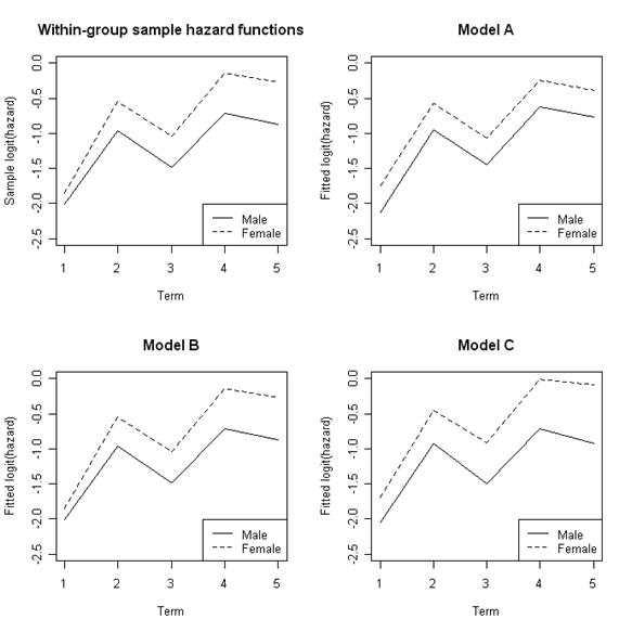
Figure 12.8, page 458. This example compares the hazard rates of male and female subjects across time for unfitted values, and then for fitted values from several different models. Note that it would be possible to generate all of these fitted and unfitted values in a single loop after running the three models. We have opted to keep these steps separate for easier reading.
math<-read.table("https://stats.idre.ucla.edu/stat/examples/alda/mathdropout_pp.csv", sep=",", header=T)
First, for each combination of time and sex, we use a loop to generate the proportion of subjects experiencing the event and calculate the logit of the proportion. Then we subset this proportion and logit data by sex.
percents <- c()
for (i in 1:5){
  for (j in 0:1){
    x <- subset(math, PERIOD==i & FEMALE==j)
    if (sum(x$EVENT) > 0){
      y <- mean(x$EVENT)}
    if (sum(x$EVENT)==0){
      y <- NA}
    logity <- log(y/(1-y))
    z <- c(i, j, y, logity)
    percents <- rbind(percents, z)}}

colnames(percents) <- c("term", "female", "pct", "logit")
percents <- as.data.frame(na.omit(percents))

percents.m <- subset(percents, female==0)
percents.f <- subset(percents, female==1)
Next, we run the first of three models, Model A. Then, using a loop, we generate predicted proportion values for each combination of time and sex with the coefficients from Model A and calculate the logit of the fitted proportion. Then we subset this proportion and logit data by sex.
modelA<-glm(EVENT ~ HS11 + HS12 + COLL1 + COLL2 + COLL3 + FEMALE - 1,
  family=binomial(link = "logit"), data = math)

modelfitA <- c()
for (i in 1:5){
  for (j in 0:1){
    logitfit <- modelA$coef[i] + modelA$coef[6]*j
    hazard = 1/(1 + exp(-logitfit))
    z <- c(i, j, logitfit, hazard)
    modelfitA <- rbind(modelfitA, z)}}

colnames(modelfitA) <- c("term", "female", "logitfit", "hazard")
modelfitA <- as.data.frame(modelfitA)
modelfitA.m <- subset(modelfitA, female==0)
modelfitA.f <- subset(modelfitA, female==1)
Next, we run the second of three models, Model B, and go through the same steps as for Model A.
modelB <- glm(EVENT ~ HS11 + HS12 + COLL1 + COLL2 + COLL3 + FHS11 + FHS12 + FCOLL1 + FCOLL2 + FCOLL3 - 1,
  family=binomial(link = "logit"), data = math)
modelfitB <- c()
for (i in 1:5){
  for (j in 0:1){
    logitfit <- modelB$coef[i] + modelB$coef[i+5]*j
    hazard = 1/(1 + exp(-logitfit))
    z <- c(i, j, logitfit, hazard)
    modelfitB <- rbind(modelfitB, z)}}

colnames(modelfitB) <- c("term", "female", "logitfit", "hazard")
modelfitB <- as.data.frame(modelfitB)
modelfitB.m <- subset(modelfitB, female==0)
modelfitB.f <- subset(modelfitB, female==1)
Next, we run the last of three models, Model C, and go through the same steps as for Model A and Model B.
modelC <- glm(EVENT ~ HS11 + HS12 + COLL1 + COLL2 + COLL3 + FEMALE + FLTIME - 1,
  family=binomial(link = "logit"), data = math)

modelfitC <- c()
for (i in 1:5){
  for (j in 0:1){
    logitfit <- modelC$coef[i] + modelC$coef[6]*j + modelC$coef[7]*i*j
    hazard = 1/(1 + exp(-logitfit))
    z <- c(i, j, logitfit, hazard)
    modelfitC <- rbind(modelfitC, z)}}

colnames(modelfitC) <- c("term", "female", "logitfit", "hazard")
modelfitC <- as.data.frame(modelfitC)
modelfitC.m <- subset(modelfitC, female==0)
modelfitC.f <- subset(modelfitC, female==1)
Lastly, we create four plots: one for the unfitted hazard and one for each of the three fitted hazards. For each graph, we start by plotting one line for males and then overlay a line for females.
par(mfrow=c(2,2))

plot(percents.m$term, percents.m$logit, type = "l", lty = 1, ylim = c(-2.5, 0),
main = "Within-group sample hazard functions", xlab = "Term", ylab = "Sample logit(hazard)")
points(percents.f$term, percents.f$logit, type = "l", lty = 2)
legend("bottomright", c("Male", "Female"), lty = c(1, 2))


plot(modelfitA.m$term, modelfitA.m$logitfit, type = "l", lty = 1, ylim = c(-2.5, 0),
main = "Model A", xlab = "Term", ylab = "Fitted logit(hazard)")
points(modelfitA.f$term, modelfitA.f$logitfit, type = "l", lty = 2)
legend("bottomright", c("Male", "Female"), lty = c(1, 2))

plot(modelfitB.m$term, modelfitB.m$logitfit, type = "l", lty = 1, ylim = c(-2.5, 0),
main = "Model B", xlab = "Term", ylab = "Fitted logit(hazard)")
points(modelfitB.f$term, modelfitB.f$logitfit, type = "l", lty = 2)
legend("bottomright", c("Male", "Female"), lty = c(1, 2))


plot(modelfitC.m$term, modelfitC.m$logitfit, type = "l", lty = 1, ylim = c(-2.5, 0),
main = "Model C", xlab = "Term", ylab = "Fitted logit(hazard)")
points(modelfitC.f$term, modelfitC.f$logitfit, type = "l", lty = 2)
legend("bottomright", c("Male", "Female"), lty = c(1, 2))
Table 12.5, page 459. The parameter estimates and fit statistics in this table can be found in the output from each of the three models below.
modelA<-glm(EVENT ~ HS11 + HS12 + COLL1 + COLL2 + COLL3 + FEMALE - 1,
family=binomial(link = "logit"), data = math)
summary(modelA)

Coefficients:
       Estimate Std. Error z value Pr(>|z|)
HS11   -2.13080    0.05674 -37.555  < 2e-16 ***
HS12   -0.94248    0.04789 -19.681  < 2e-16 ***
COLL1  -1.44948    0.06345 -22.845  < 2e-16 ***
COLL2  -0.61765    0.07571  -8.158 3.42e-16 ***
COLL3  -0.77160    0.14280  -5.403 6.54e-08 ***
FEMALE  0.37865    0.05015   7.551 4.33e-14 ***
---
Signif. codes:  0 '***' 0.001 '**' 0.01 '*' 0.05 '.' 0.1 ' ' 1

(Dispersion parameter for binomial family taken to be 1)

    Null deviance: 13250.2  on 9558  degrees of freedom
Residual deviance:  9804.3  on 9552  degrees of freedom
AIC: 9816.3
modelB <- glm(EVENT ~ HS11 + HS12 + COLL1 + COLL2 + COLL3 + FHS11 + FHS12 + FCOLL1 + FCOLL2 + FCOLL3 - 1,
family=binomial(link = "logit"), data = math)
summary(modelB)

Coefficients:
       Estimate Std. Error z value Pr(>|z|)
HS11   -2.00767    0.07148 -28.087  < 2e-16 ***
HS12   -0.96425    0.05854 -16.470  < 2e-16 ***
COLL1  -1.48240    0.08471 -17.499  < 2e-16 ***
COLL2  -0.71001    0.10073  -7.048 1.81e-12 ***
COLL3  -0.86904    0.19077  -4.555 5.23e-06 ***
FHS11   0.15680    0.09777   1.604 0.108791
FHS12   0.41866    0.07924   5.284 1.27e-07 ***
FCOLL1  0.44068    0.11580   3.805 0.000142 ***
FCOLL2  0.57075    0.14455   3.948 7.86e-05 ***
FCOLL3  0.60077    0.28573   2.103 0.035502 *
---
Signif. codes:  0 '***' 0.001 '**' 0.01 '*' 0.05 '.' 0.1 ' ' 1

(Dispersion parameter for binomial family taken to be 1)

    Null deviance: 13250.2  on 9558  degrees of freedom
Residual deviance:  9796.3  on 9548  degrees of freedom
AIC: 9816.3
modelC <- glm(EVENT ~ HS11 + HS12 + COLL1 + COLL2 + COLL3 + FEMALE + FLTIME - 1,
family=binomial(link = "logit"), data = math)
summary(modelC)
Coefficients:
       Estimate Std. Error z value Pr(>|z|)
HS11   -2.04592    0.06464 -31.649  < 2e-16 ***
HS12   -0.92551    0.04821 -19.197  < 2e-16 ***
COLL1  -1.49655    0.06649 -22.507  < 2e-16 ***
COLL2  -0.71781    0.08605  -8.341  < 2e-16 ***
COLL3  -0.91655    0.15570  -5.887 3.94e-09 ***
FEMALE  0.22749    0.07744   2.937  0.00331 **
FLTIME  0.11977    0.04698   2.549  0.01080 *
---
Signif. codes:  0 '***' 0.001 '**' 0.01 '*' 0.05 '.' 0.1 ' ' 1

(Dispersion parameter for binomial family taken to be 1)

    Null deviance: 13250.2  on 9558  degrees of freedom
Residual deviance:  9797.8  on 9551  degrees of freedom
AIC: 9811.8
Table 12.6, page 465. This table shows some summary information for a set of eight subjects. To generate this table in R, we wrote a function that takes an ID number as an argument and returns a vector containing the information seen in a given row of this table.
firstsex<-read.table("https://stats.idre.ucla.edu/stat/examples/alda/firstsex_pp.csv", sep=",", header=T)
First, we fit a logistic model to the data predicting the event using time, PT, and PAS. From this model, we then generated a deviance residual for each observation.
model12.6<-glm(event ~ d7 + d8 + d9 + d10 + d11 + d12 + pt+pas- 1, family=binomial(link = "logit"), data = firstsex)
firstsex.r <- cbind(firstsex, dev.res = residuals(model12.6, type="deviance"))
Next, we defined a function that limits the dataset to a given subject, and then extracts the subjects last (greatest time point value) values for PT, PAS, grade, and censor. The function then creates a vector containing this information, the deviance residuals from all the time points for which the subject has data, and an SS deviance for the subject.
get12.6 <- function(id.num){
  x <- subset(firstsex.r, id==id.num)
  pt <- max(x$pt)
  pas <- max(x$pas)
  grade <- max(x$period)
  censor <- abs(max(x$event)-1)
  gr <- x$dev.res
  gr.l <- length(gr)
  if (gr.l < 6){
    gr <- c(gr, c(rep(NA, (6-gr.l))))}
  ss.dev <- sum(na.omit(gr*gr))
  z <- c(id.num, pt, pas, grade, censor, gr, ss.dev)
  return(z)}
The table was created by calling the above function with the eight IDs that appear in the table and stacking the eight vectors together.
tab12.6 <- rbind(get12.6(22), get12.6(112), get12.6(166), get12.6(89), get12.6(102), get12.6(87), get12.6(67), get12.6(212))
colnames(tab12.6) <- c("id", "pt", "pas", "grade", "censor", "gr7", "gr8", "gr9", "gr10", "gr11", "gr12", "ss.dev")

tab12.6

      id pt        pas grade censor        gr7        gr8        gr9       gr10       gr11       gr12   ss.dev
[1,]  22  1 -0.6496482    12      0 -0.4117311 -0.2944395 -0.5840395 -0.7176492 -0.7747741  1.4144633 3.713321
[2,] 112  1 -0.6609311    12      1 -0.4110716 -0.2939581 -0.5831423 -0.7165919 -0.7736556 -0.9562858 2.621976
[3,] 166  1  2.7814130    11      0 -0.6614533 -0.4806816 -0.9108230 -1.0903113  1.1913978         NA 4.106381
[4,]  89  0 -0.0751572    11      0 -0.3248377 -0.2313901 -0.4644566 -0.5751775  1.8623690         NA 4.174028
[5,] 102  1  0.6049317     8      0 -0.4913390  2.3694820         NA         NA         NA         NA 5.855859
[6,]  87  1  2.6779010     7      0  1.8176297         NA         NA         NA         NA         NA 3.303778
[7,]  67  1  2.2746520    12      0 -0.6180257 -0.4476515 -0.8559141 -1.0294308 -1.1007321  1.0429686 4.674059
[8,] 212  0 -0.9617912    12      1 -0.2857033 -0.2032141 -0.4097550 -0.5090181 -0.5524318 -0.6958426 1.339299
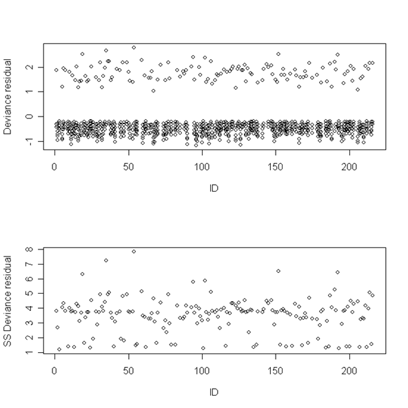
Figure 12.8, page 467. These two plots are generated using the deviance residuals from a model. The first plot depicts the residuals from all of the observations, while the second depicts the sum of squared residuals for each ID. We first need to fit the model and generate the residuals.
firstsex<-read.table("https://stats.idre.ucla.edu/stat/examples/alda/firstsex_pp.csv", sep=",", header=T)
model12.6<-glm(event ~ d7 + d8 + d9 + d10 + d11 + d12 + pt+pas- 1, family=binomial(link = "logit"), data = firstsex)
firstsex.r <- cbind(firstsex, dev.res = residuals(model12.6, type="deviance"))
Next, we have defined a function that accepts an ID as an argument and calculates the sum of the squared deviance residuals for observations associated with the given ID.
get12.9 <- function(id.num){
  x <- subset(firstsex.r, id==id.num)
  gr <- x$dev.res
  ss.dev <- sum((gr*gr))
  return(ss.dev)}
Having defined the above function, we loop through the values of ID, calling the above function to calculate the sum of squared residuals for each ID. This gives us a dataset containing one observation per ID.
ss.devs <- c()
  for (i in 1:216){
  z <- c(i, get12.9(i))
  if (z[2]!=0){
    ss.devs <- rbind(ss.devs, z)}}
Finally, we create two plots: one of all of the deviance residuals against ID and one of the sum of squared residuals against ID.
par(mfrow=c(2,1))
plot(firstsex.r$id, firstsex.r$dev.res, ylab = "Deviance residual", xlab = "ID")
plot(ss.devs[,1], ss.devs[,2], ylab = "SS Deviance residual", xlab = "ID")

