Applied Longitudinal Data Analysis: Modeling Change and Event Occurrence by Judith D. Singer and John B. Willett Chapter 13: Describing Continuous-Time Event Occurrence Data
The examples on the page were written in R version 2.4.1. This page requires the R package survival.
library(survival)
Table 13.2, page 477. To generate this table, we will determine which observations fall into which intervals presented in the table, and then calculate the estimates using the counts at each interval.
honk<-read.table("https://stats.idre.ucla.edu/stat/examples/alda/honking.csv", sep=",", header=T)
First, we define the intervals and determine the number at risk, the number of events, and the number of censored observations for each interval.
interval<- rep(dim(honk)[1], 0)
for (i in 1:dim(honk)[1]){
  interval[i] = min(floor(honk$SECONDS[i]), 8)}

int.event <- rep(0, 8)
int.censor <- rep(0, 8)
for (i in 1:dim(honk)[1]){
  int <- interval[i]
  if (honk$CENSOR[i] == 0) int.event[int] <- int.event[int]+1
  if (honk$CENSOR[i] == 1) int.censor[int] <- int.censor[int] + 1}

interval <- c(1:8)
interval.end <- c(2:8, 18)
interval.w <- interval.end - interval

int.risk <- c(57, rep(0, 7))
for (i in 2:8){
  int.risk[i] <- int.risk[i-1] - (int.event[i-1] + int.censor[i-1])}
Next, we can calculate the conditional probability of the event in each interval and the discrete and actuarial hazard rates.
phat = (int.event/int.risk)
discrete.h = (phat/interval.w)
actuarial.h = (int.event/(int.risk - (int.censor/2) - (int.event/2)))/interval.w
Using the hazard rates for each interval, we can calculate the discrete and actuarial survival rates. The formulas for these are found in the text.
discrete.s <- c(1-discrete.h[1], rep(0, 7))
actuarial.s <- c((1-5/(57-1/2)), rep(0,7))
for (i in 2:8){
  discrete.s[i] <- (1 - phat[i])*discrete.s[i-1]
  actuarial.s[i] <- actuarial.s[i-1]*(1-int.event[i]/(int.risk[i] - int.censor[i]/2))}
Lastly, we combine all of these interval measures into one table.
int.table <- cbind(interval, interval.end, int.risk, int.event, int.censor, phat, discrete.s, discrete.h, actuarial.s, actuarial.h)
int.table
     interval interval.end int.risk int.event int.censor      phat discrete.s discrete.h actuarial.s actuarial.h
[1,]        1            2       57         5          1 0.0877193 0.91228070  0.0877193  0.91150442   0.0925926
[2,]        2            3       51        14          3 0.2745098 0.66185071  0.2745098  0.65370519   0.3294118
[3,]        3            4       34         9          2 0.2647059 0.48665493  0.2647059  0.47542196   0.3157895
[4,]        4            5       23         6          4 0.2608696 0.35970147  0.2608696  0.33958711   0.3333333
[5,]        5            6       13         2          2 0.1538462 0.30436278  0.1538462  0.28298926   0.1818182
[6,]        6            7        9         2          2 0.2222222 0.23672661  0.2222222  0.21224195   0.2857143
[7,]        7            8        5         1          0 0.2000000 0.18938129  0.2000000  0.16979356   0.2222222
[8,]        8           18        4         3          1 0.7500000 0.04734532  0.0750000  0.02425622   0.1500000
Figure 13.1, page 479. For this example, we will start from the table we created in the previous example. For the actuarial graphs, we can use the R function stepfun to create a data object that, when plotted, appears as a step function.
attach(data.frame(int.table))
par(mfrow=c(2,2))

plot(c(0, interval.end), c(1,discrete.s), type = "l", xlim = c(0, 20), ylim = c(0,1),
  ylab = "Discrete Survival", xlab = "Seconds after light turns green")
s.hat.steps <- stepfun(interval, c(1, actuarial.s))
plot(s.hat.steps, do.points = FALSE, xlim = c(0, 20),
  ylab = "Actuarial Survival", xlab = "Seconds after light turns green", main = "")

plot(interval.end, discrete.h, type = "l", xlim = c(0, 20), ylim = c(0, .35),
  ylab = "Discrete Hazard", xlab = "Seconds after light turns green")

h.hat.steps <- stepfun(interval, c(NA, actuarial.h))
plot(h.hat.steps, do.points = FALSE, xlim = c(0, 20), ylim = c(0, .35),
  ylab = "Actuarial Hazard", xlab = "Seconds after light turns green", main = "")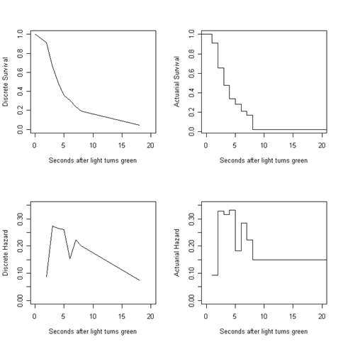
Table 13.3, page 484. To generate this table, we start by using the survfit and Surv commands from the R survival package.
t13.3 <- summary(survfit(Surv(honk$SECONDS, abs(honk$CENSOR - 1))~1))
From the survival fit, we are only interested in a specific set of columns which we rename below.
s.hat <- t13.3$surv
time <- t13.3$time
n.atrisk <- t13.3$n.risk
n.events <- t13.3$n.event
se.s.hat <- t13.3$std.err

n.censored <- width <- p.hat <- rep(0, length(t13.3$surv))
We can generate the conditional probability of the event, the width, and the number of censored observations for each interval.
for (i in 1:(length(t13.3$surv))){
 p.hat[i] <- n.events[i] / n.atrisk[i]
 if (i < (length(t13.3$surv))){
 n.censored[i] <- (n.atrisk[i]-n.atrisk[i+1]) - n.events[i]
 width[i] <- time[i+1] - time[i]}
 if (i == (length(t13.3$surv))){
 n.censored[i] <- (n.atrisk[i]- n.events[i])
 width[i] <- NA}}

h.hat <- p.hat/width
Lastly, we combine all of these interval measures into one table.
tab13.3 <- cbind(time, n.atrisk, n.events, n.censored, p.hat, s.hat, se.s.hat, width, h.hat)
tab13.3
       time n.atrisk n.events n.censored      p.hat      s.hat   se.s.hat width      h.hat
 [1,]  1.41       57        1          1 0.01754386 0.98245614 0.01738929  0.10 0.17543860
 [2,]  1.51       55        1          0 0.01818182 0.96459330 0.02459209  0.16 0.11363636
 [3,]  1.67       54        1          0 0.01851852 0.94673046 0.02992911  0.01 1.85185185
 [4,]  1.68       53        1          0 0.01886792 0.92886762 0.03428307  0.18 0.10482180
 [5,]  1.86       52        1          0 0.01923077 0.91100478 0.03799347  0.26 0.07396450
 [6,]  2.12       51        1          0 0.01960784 0.89314195 0.04123439  0.07 0.28011204
 [7,]  2.19       50        1          1 0.02000000 0.87527911 0.04410945  0.29 0.06896552
 [8,]  2.48       48        1          0 0.02083333 0.85704413 0.04680819  0.02 1.04166667
 [9,]  2.50       47        1          0 0.02127660 0.83880914 0.04923621  0.03 0.70921986
[10,]  2.53       46        1          0 0.02173913 0.82057416 0.05143185  0.01 2.17391304
[11,]  2.54       45        1          0 0.02222222 0.80233918 0.05342379  0.02 1.11111111
[12,]  2.56       44        1          0 0.02272727 0.78410420 0.05523405  0.06 0.37878788
[13,]  2.62       43        1          0 0.02325581 0.76586922 0.05688000  0.06 0.38759690
[14,]  2.68       42        1          2 0.02380952 0.74763424 0.05837553  0.15 0.15873016
[15,]  2.83       39        1          0 0.02564103 0.72846413 0.05994380  0.05 0.51282051
[16,]  2.88       38        1          0 0.02631579 0.70929402 0.06135512  0.01 2.63157895
[17,]  2.89       37        1          0 0.02702703 0.69012391 0.06262011  0.03 0.90090090
[18,]  2.92       36        1          0 0.02777778 0.67095380 0.06374747  0.06 0.46296296
[19,]  2.98       35        1          1 0.02857143 0.65178369 0.06474439  0.16 0.17857143
[20,]  3.14       33        1          0 0.03030303 0.63203267 0.06572607  0.03 1.01010101
[21,]  3.17       32        1          0 0.03125000 0.61228165 0.06657366  0.04 0.78125000
[22,]  3.21       31        1          0 0.03225806 0.59253063 0.06729223  0.01 3.22580645
[23,]  3.22       30        1          0 0.03333333 0.57277961 0.06788588  0.02 1.66666667
[24,]  3.24       29        1          1 0.03448276 0.55302859 0.06835785  0.32 0.10775862
[25,]  3.56       27        1          0 0.03703704 0.53254605 0.06882637  0.01 3.70370370
[26,]  3.57       26        1          0 0.03846154 0.51206351 0.06915985  0.01 3.84615385
[27,]  3.58       25        1          0 0.04000000 0.49158097 0.06936025  0.20 0.20000000
[28,]  3.78       24        1          1 0.04166667 0.47109843 0.06942872  0.32 0.13020833
[29,]  4.10       22        1          0 0.04545455 0.44968486 0.06949670  0.08 0.56818182
[30,]  4.18       21        1          1 0.04761905 0.42827130 0.06940798  0.26 0.18315018
[31,]  4.44       19        1          0 0.05263158 0.40573070 0.06931846  0.07 0.75187970
[32,]  4.51       18        1          0 0.05555556 0.38319011 0.06903504  0.01 5.55555556
[33,]  4.52       17        1          2 0.05882353 0.36064951 0.06855532  0.44 0.13368984
[34,]  4.96       14        1          1 0.07142857 0.33488883 0.06832728  0.43 0.16611296
[35,]  5.39       12        1          0 0.08333333 0.30698143 0.06809447  0.34 0.24509804
[36,]  5.73       11        1          1 0.09090909 0.27907403 0.06738052  0.30 0.30303030
[37,]  6.03        9        1          1 0.11111111 0.24806580 0.06664790  0.27 0.41152263
[38,]  6.30        7        1          1 0.14285714 0.21262783 0.06587800  0.90 0.15873016
[39,]  7.20        5        1          0 0.20000000 0.17010227 0.06499447  2.39 0.08368201
[40,]  9.59        4        1          0 0.25000000 0.12757670 0.06109400  2.70 0.09259259
[41,] 12.29        3        1          0 0.33333333 0.08505113 0.05352097  0.89 0.37453184
[42,] 13.18        2        1          1 0.50000000 0.04252557 0.04025339    NA         NA
Figure 13.2, page 485. For the first graph, we will generate a step function using the Kaplan-Meier estimated survival from the previous table and plot it.
par(mfrow=c(2,1))
s.hat.steps <- stepfun(time, c(1, s.hat))
plot(s.hat.steps, do.points = FALSE, xlim = c(0, 20), ylim = c(0,1),
  ylab = "Estimated Survival", xlab = "Seconds after light turns green", main = "")
For the second graph, we start with the same step survival function as the first graph.
plot(s.hat.steps, do.points = FALSE, xlim = c(0, 20), ylim = c(0,1),
  ylab = "Estimated Survival", xlab = "Seconds after light turns green", main = "")
Then we overlay the actuarial and discrete-time survival estimates using the imposed intervals from Table 13.2.
attach(data.frame(int.table))
points(c(1, interval.end), c(1, discrete.s), type = "l", lty = 2)
s.hat.actuarial <- stepfun(c(interval, 18), c(1, actuarial.s, 0.02425622))
lines(s.hat.actuarial , do.points = FALSE, lty = 3)
legend("topright", c("Kaplan-Meier", "Discrete Time", "Actuarial"), lty = c(1, 2, 3))
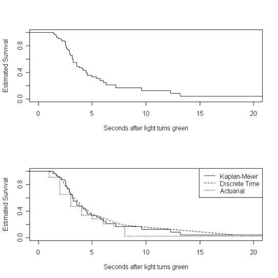
Figure 13.4, page 493. We have only generated the first of the two graphs in this figure. The second is identical to the first, but with estimated line functions added. For this graph, we first calculated both the negative log of the survival estimate and the Nelson-Aalen estimate of the cumulative hazard. Then, we generated step functions for both overlayed one over the other (using lines rather than the usual points command for overlays in R).
nl.s <- -log(s.hat)
nls.steps <- stepfun(time, c(0, nl.s))

NA.est <- c(0, rep(0, length(s.hat)))
for (i in 2:length(NA.est)){
  NA.est[i] <- NA.est[i-1]+p.hat[i-1]}

NA.steps <- stepfun(time, NA.est)

par(mfrow=c(1,1))
plot(nls.steps, do.points = FALSE, xlim = c(0, 20), ylim = c(0,3.5),
  ylab = "Cumulative Hazard", xlab = "Seconds after light turns green", main = "")
lines(NA.steps, do.points = FALSE, lty =2, xlim = c(0,20))
legend("bottomright", c("Negative Log Survival", "Nelson-Aalen"), lty = c(1, 2))
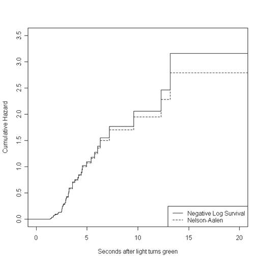
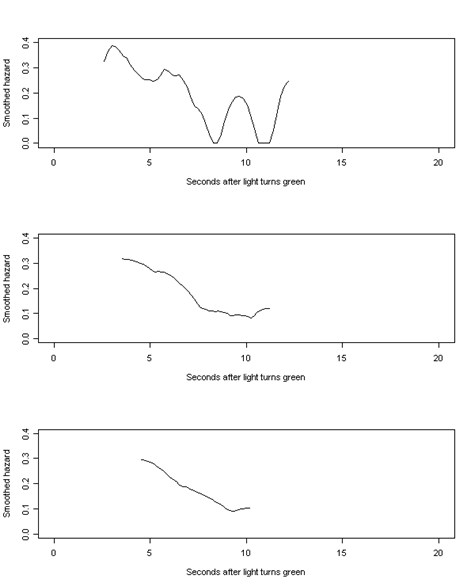
Figure 13.5, page 496. We have generated these graphs by first writing a function smooth that takes the time and estimated survival probabilities from the survfit in an earlier example and aggregates hazard over a given width of time. This function was written using the same smoothing algorithm the authors used. If we were to use one of R’s kernel smoothing functions (like ksmooth), we would not be able to exactly reproduce the graphs as they appear in the text.
smooth<- function(width, time, survive){
n=length(time)
lo=time[1] + width
hi=time[n] - width
npt=50
inc=(hi-lo)/npt
s=lo+t(c(1:npt))*inc
slag = c(1, survive[1:n-1])
h=1-survive/slag
x1 = as.vector(rep(1, npt))%*%(t(time))
x2 = t(s)%*%as.vector(rep(1,n))
x = (x1 - x2) / width
k=.75*(1-x*x)*(abs(x)<=1)
lambda=(k%*%h)/width
smoothed= list(x = s, y = lambda)
return(smoothed)
}

par(mfrow=c(3,1))
bw1 <- smooth(1, time, s.hat)
plot(bw1$x, bw1$y, type = "l", xlim = c(0, 20), ylim = c(0, .4),
  xlab = "Seconds after light turns green", ylab = "Smoothed hazard")
bw2 <- smooth(2, time, s.hat)
plot(bw2$x, bw2$y, type = "l", xlim = c(0, 20), ylim = c(0, .4),
  xlab = "Seconds after light turns green", ylab = "Smoothed hazard")
bw3 <- smooth(3, time, s.hat)
plot(bw3$x, bw3$y, type = "l", xlim = c(0, 20), ylim = c(0, .4),
  xlab = "Seconds after light turns green", ylab = "Smoothed hazard")
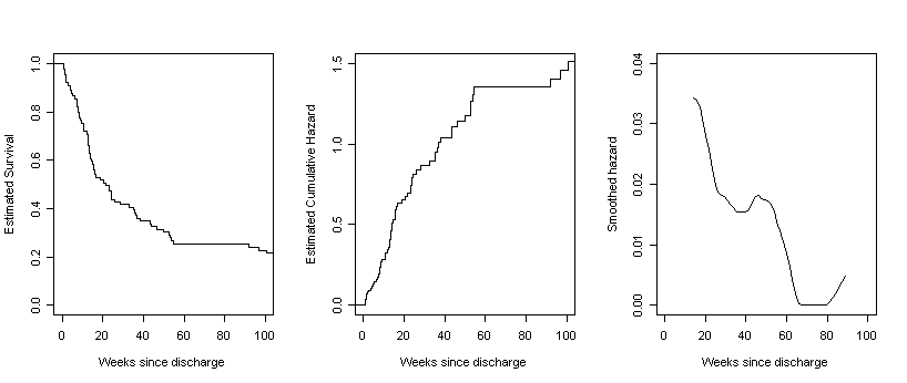
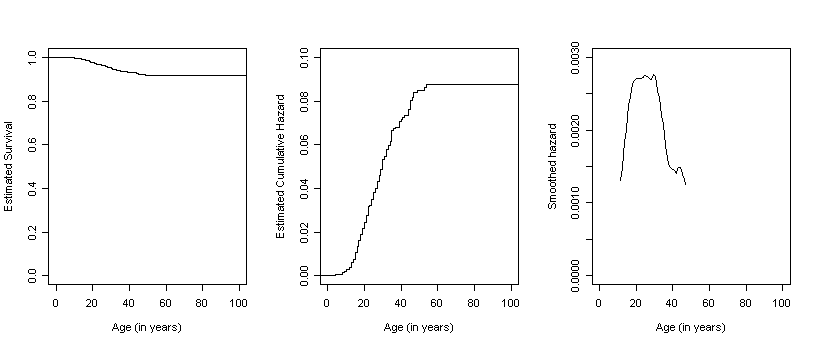
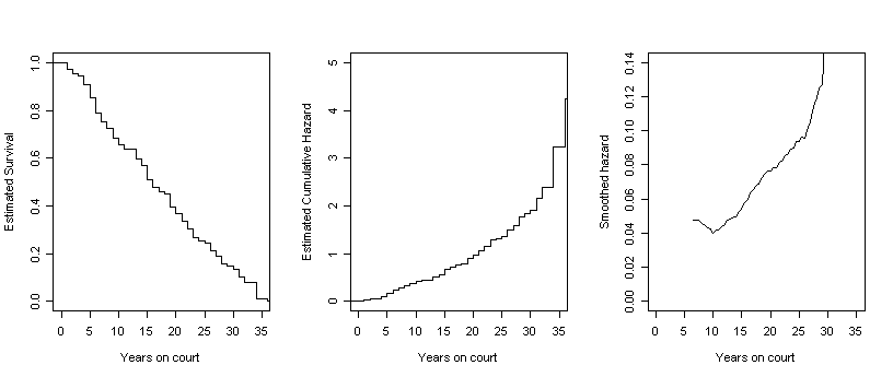
Figure 13.6, page 499. For each column of three graphs, we have created the first two by generating step functions of survival and cumulative hazard rates and then used the smooth function defined earlier in this page to generate the data for the third graph, a smoothed hazard. For each of the four datasets in this example, we began by generating the survival estimates, time, and conditional probability estimates using the summary of the survival fit. We then calculate the Nelson-Aalen estimates by looping through the interval data and ran the smooth function.
relapse<-read.table("https://stats.idre.ucla.edu/stat/examples/alda/alcohol_relapse.csv", sep=",", header=T)
judges<-read.table("https://stats.idre.ucla.edu/stat/examples/alda/judges.csv", sep=",", header=T)
depression<-read.table("https://stats.idre.ucla.edu/stat/examples/alda/firstdepression.csv", sep=",", header=T)
hw<-read.table("https://stats.idre.ucla.edu/stat/examples/alda/healthworkers.csv", sep=",", header=T)
f13.6A <- summary(survfit(Surv(relapse$WEEKS, abs(relapse$CENSOR - 1))~1))
s.hat.A <- f13.6A$surv
time.A <- f13.6A$time
phat.A <- (f13.6A[4][[1]] / f13.6A[3][[1]])
NA.est.A <- c(0, rep(0, length(s.hat.A)))
width.A <- c(0, length(s.hat.A)-1)
for (i in 2:length(NA.est.A)){
  NA.est.A[i] <- NA.est.A[i-1]+phat.A[i-1]}

stepsA.h <- stepfun(time.A, NA.est.A)
stepsA.s <- stepfun(time.A, c(1,s.hat.A))
smooth.A <- smooth(12, time.A, s.hat.A)

par(mfrow=c(1,3))
plot(stepsA.s, do.points = FALSE, xlim = c(0,100), ylim = c(0,1),
  xlab = "Weeks since discharge", ylab = "Estimated Survival", main = "")
plot(stepsA.h, do.points = FALSE, xlim = c(0,100), ylim = c(0,1.5),
  xlab = "Weeks since discharge", ylab = "Estimated Cumulative Hazard", main = "")
plot(smooth.A$x, smooth.A$y, type = "l", xlim = c(0, 100), ylim = c(0, .04),
  xlab = "Weeks since discharge", ylab = "Smoothed hazard")
f13.6B <- summary(survfit(Surv(judges$tenure, judges$leave)~1))
s.hat.B <- f13.6B$surv
time.B <- f13.6B$time
phat.B <- (f13.6B[4][[1]] / f13.6B[3][[1]])
NA.est.B <- c(0, rep(0, length(s.hat.B)))
for (i in 2:length(NA.est.B)){
  NA.est.B[i] <- NA.est.B[i-1]+phat.B[i-1]}
stepsB.h <- stepfun(time.B, NA.est.B)
stepsB.s <- stepfun(time.B, c(1,s.hat.B))
smooth.B <- smooth(5, time.B, s.hat.B)

plot(stepsB.s, do.points = FALSE, xlim = c(0,35), ylim = c(0,1),
  xlab = "Years on court", ylab = "Estimated Survival", main = "")
plot(stepsB.h, do.points = FALSE, xlim = c(0,35), ylim = c(0,5),
  xlab = "Years on court", ylab = "Estimated Cumulative Hazard", main = "")
plot(smooth.B$x, smooth.B$y, type = "l", xlim = c(0, 35), ylim = c(0, .14),
  xlab = "Years on court", ylab = "Smoothed hazard")
f13.6C <- summary(survfit(Surv(depression$age, abs(depression$censor - 1))~1))

s.hat.C <- f13.6C$surv
time.C <- f13.6C$time
phat.C <- (f13.6C[4][[1]] / f13.6C[3][[1]])
NA.est.C <- c(0, rep(0, length(s.hat.C)))
for (i in 2:length(NA.est.C)){
  NA.est.C[i] <- NA.est.C[i-1]+phat.C[i-1]}

stepsC.h <- stepfun(time.C, NA.est.C)
stepsC.s <- stepfun(time.C, c(1,s.hat.C))
smooth.C <- smooth(7, time.C, s.hat.C)

plot(stepsC.s, do.points = FALSE, xlim = c(0,100), ylim = c(0,1),
  xlab = "Age (in years)", ylab = "Estimated Survival", main = "")
plot(stepsC.h, do.points = FALSE, xlim = c(0,100), ylim = c(0,.1),
  xlab = "Age (in years)", ylab = "Estimated Cumulative Hazard", main = "")
plot(smooth.C$x, smooth.C$y, type = "l", xlim = c(0, 100), ylim = c(0, .003),
  xlab = "Age (in years)", ylab = "Smoothed hazard")
f13.6D <- summary(survfit(Surv(hw$weeks, abs(hw$censor - 1))~1))

s.hat.D <- f13.6D$surv
time.D <- f13.6D$time
phat.D <- (f13.6D[4][[1]] / f13.6D[3][[1]])
NA.est.D <- c(0, rep(0, length(s.hat.D)))
for (i in 2:length(NA.est.D)){
  NA.est.D[i] <- NA.est.D[i-1]+phat.D[i-1]}
stepsD.h <- stepfun(time.D, NA.est.D)
stepsD.s <- stepfun(time.D, c(1,s.hat.D))
smooth.D <- smooth(7, time.D, s.hat.D)

plot(stepsD.s, do.points = FALSE, xlim = c(0,145), ylim = c(0,1),
  xlab = "Weeks since hired", ylab = "Estimated Survival", main = "")
plot(stepsD.h, do.points = FALSE, xlim = c(0,145), ylim = c(0,.6),
  xlab = "Weeks since hired", ylab = "Estimated Cumulative Hazard", main = "")
plot(smooth.D$x, smooth.D$y, type = "l", xlim = c(0, 145), ylim = c(0, .011),
  xlab = "Weeks since hired", ylab = "Smoothed hazard")


