R Textbook Examples Applied Longitudinal Data Analysis: Modeling Change and Event Occurrence by Judith D. Singer and John B. Willett
Chapter 15: Extending the Cox Regression Model
Note: All code and notes on this page were written by Llewellyn Mills, PhD. We sincerely thank Llew for generously offering his code, which completes the Applied Longitudinal Data Analysis examples for R, to put up on our website. Email llewmills@gmail.com for questions about the code.
This page requires the R packages survival and ggplot2
library(survival)
library(ggplot2)
Table 15.1 p.548
cocaine <- read.csv("https://stats.idre.ucla.edu/stat/examples/alda/firstcocaine.csv")First create an EVENT variable
cocaine$EVENT <- 1 - cocaine$CENSORNext create a reduced version of the dataset with only the variables we need.
cocaine <- cocaine[, c("ID", "BIRTHYR", "COKEAGE", "EARLYMJ", "EARLYOD",
                       "EVENT", "MJAGE", "ODAGE", "SELLMJAGE", "SDAGE")]
Model A
Model A is a simple cox regression, with COKEAGE as the time indicator and EVENT as the indicator of whether the event (or censorship) occurred.
modA <- coxph(Surv(COKEAGE, EVENT) ~ BIRTHYR + EARLYMJ + EARLYOD, data = cocaine)
summary(modA)
## Call:
## coxph(formula = Surv(COKEAGE, EVENT) ~ BIRTHYR + EARLYMJ + EARLYOD,
## data = cocaine)
##
## n= 1658, number of events= 382
##
## coef exp(coef) se(coef) z Pr(>|z|)
## BIRTHYR 0.15508 1.16776 0.01993 7.782 7.11e-15 ***
## EARLYMJ 1.21707 3.37729 0.16403 7.420 1.17e-13 ***
## EARLYOD 0.79117 2.20599 0.19620 4.032 5.52e-05 ***
## ---
## Signif. codes: 0 '***' 0.001 '**' 0.01 '*' 0.05 '.' 0.1 ' ' 1
##
## exp(coef) exp(-coef) lower .95 upper .95
## BIRTHYR 1.168 0.8563 1.123 1.214
## EARLYMJ 3.377 0.2961 2.449 4.658
## EARLYOD 2.206 0.4533 1.502 3.240
##
## Concordance= 0.707 (se = 0.015 )
## Rsquare= 0.139 (max possible= 0.964 )
## Likelihood ratio test= 247.8 on 3 df, p=0
## Wald test = 317.9 on 3 df, p=0
## Score (logrank) test = 445.7 on 3 df, p=0Model B
In model B we replace the two time-invariant measures of drug use, EARLYMJ and EARLYOD with their time-varying cousins MJAGE and ODAGE. Because the survival package uses a single-entry method we need to create a count-process dataset (i.e. a person-period, long-form dataset). To do this we need to alter the dataset so that there are rows for every interval when one of the covariates occurred to anyone in the sample. We create the count process dataset using the tmerge() function in the survival package. The tmerge function requires two datasets as its first two arguments, however you can specify the same dataset twice (this may not make sense reading it now but see below). It also requires an id = argument, specifying the id variable (in our case ID). Next is the crucial argument, event(), which creates the tstart and tstop variables. The event() argument itself has two arguments: the first in which you first specify the variable indicating time-of-event (or censoring) (here COKEAGE); the second in which you specify whether the event occurred or not (here the EVENT variable). The argument that creates the multiple rows that make it a person-period, count-process dataset is the ‘tdc()’ argument.
If an individual did not experience the covariate event in question all entries for that variable will be NA.
In this example we create two time-varying covariates: USEMJ, a time-varying variable that indicates, at each time point, each individual’s status with respect to marijuana use, and USEOD, a time-varying covariate indicating use of other drugs.
Let’s create the count-process dataset.
longModBDF <- tmerge(cocaine, cocaine,
                     id = ID,
                     start_using = event(COKEAGE, EVENT),
                     USEMJ = tdc(MJAGE),
                     USEOD = tdc(ODAGE))
Examining the new dataframe
head(longModBDF[order(longModBDF$ID),])## ID BIRTHYR COKEAGE EARLYMJ EARLYOD EVENT MJAGE ODAGE SELLMJAGE SDAGE
## 2593 5 0 41 0 0 0 23 24 NA 24
## 2594 5 0 41 0 0 0 23 24 NA 24
## 2595 5 0 41 0 0 0 23 24 NA 24
## 962 8 10 32 0 0 0 NA NA NA NA
## 2401 9 5 36 0 0 0 18 NA NA NA
## 2402 9 5 36 0 0 0 18 NA NA NA
## id tstart tstop start_using USEMJ USEOD
## 2593 5 0 23 0 0 0
## 2594 5 23 24 0 1 0
## 2595 5 24 41 0 1 1
## 962 8 0 32 0 0 0
## 2401 9 0 18 0 0 0
## 2402 9 18 36 0 1 0Now we can fit model B
modB <- coxph(Surv(tstart, tstop, start_using) ~ BIRTHYR + USEMJ + USEOD,
              data= longModBDF, ties="efron")
summary(modB)
## Call:
## coxph(formula = Surv(tstart, tstop, start_using) ~ BIRTHYR +
## USEMJ + USEOD, data = longModBDF, ties = "efron")
##
## n= 3086, number of events= 382
##
## coef exp(coef) se(coef) z Pr(>|z|)
## BIRTHYR 0.10741 1.11340 0.02145 5.008 5.5e-07 ***
## USEMJ 2.55176 12.82972 0.28095 9.082 < 2e-16 ***
## USEOD 1.85387 6.38446 0.12921 14.347 < 2e-16 ***
## ---
## Signif. codes: 0 '***' 0.001 '**' 0.01 '*' 0.05 '.' 0.1 ' ' 1
##
## exp(coef) exp(-coef) lower .95 upper .95
## BIRTHYR 1.113 0.89815 1.068 1.161
## USEMJ 12.830 0.07794 7.397 22.252
## USEOD 6.384 0.15663 4.956 8.225
##
## Concordance= 0.876 (se = 0.015 )
## Rsquare= 0.242 (max possible= 0.833 )
## Likelihood ratio test= 856 on 3 df, p=0
## Wald test = 451.1 on 3 df, p=0
## Score (logrank) test = 1039 on 3 df, p=0Models A and B aren’t nested so you can’t compare -2LL statistics (e.g. with the anova() command); however you can compare their AICs. The extractAIC() function will return the equivalent degrees of freedom for the fitted model, then the AIC.
extractAIC(modA); extractAIC(modB)## [1] 3.000 5283.228## [1] 3.000 4675.096Model C
In model C we look at the effect of two other time-varying predictors—age of first selling marijuana (SELLMJAGE), and age of first selling other drugs (SDAGE)—which we add to the two we tested in Model B—MJAGE and ODAGE. Adding more time-varying covariates means there will be more rows per individual, so we need to recreate the count process dataset.
longModCDF <-  tmerge(cocaine, cocaine,
                      id = ID,
                      start_using = event(COKEAGE, EVENT),
                      USEMJ = tdc(MJAGE),
                      USEOD = tdc(ODAGE),
                      SELLMJ = tdc(SELLMJAGE),
                      SELLOD = tdc(SDAGE))
Now fit the model.
modC <- coxph(Surv(tstart, tstop, start_using) ~ BIRTHYR + USEMJ +
                USEOD + SELLMJ + SELLOD, data= longModCDF, ties="efron")
summary(modC)
## Call:
## coxph(formula = Surv(tstart, tstop, start_using) ~ BIRTHYR +
## USEMJ + USEOD + SELLMJ + SELLOD, data = longModCDF, ties = "efron")
##
## n= 3312, number of events= 382
##
## coef exp(coef) se(coef) z Pr(>|z|)
## BIRTHYR 0.08493 1.08864 0.02183 3.890 1e-04 ***
## USEMJ 2.45920 11.69542 0.28357 8.672 < 2e-16 ***
## USEOD 1.25110 3.49419 0.15656 7.991 1.33e-15 ***
## SELLMJ 0.68989 1.99349 0.12263 5.626 1.84e-08 ***
## SELLOD 0.76037 2.13908 0.13066 5.819 5.91e-09 ***
## ---
## Signif. codes: 0 '***' 0.001 '**' 0.01 '*' 0.05 '.' 0.1 ' ' 1
##
## exp(coef) exp(-coef) lower .95 upper .95
## BIRTHYR 1.089 0.9186 1.043 1.136
## USEMJ 11.695 0.0855 6.709 20.389
## USEOD 3.494 0.2862 2.571 4.749
## SELLMJ 1.993 0.5016 1.568 2.535
## SELLOD 2.139 0.4675 1.656 2.763
##
## Concordance= 0.89 (se = 0.015 )
## Rsquare= 0.248 (max possible= 0.811 )
## Likelihood ratio test= 944.5 on 5 df, p=0
## Wald test = 594.2 on 5 df, p=0
## Score (logrank) test = 1592 on 5 df, p=0Model D
Now we run the full model.
longModDDF <- tmerge(cocaine, cocaine,
                     id = ID,
                     start_using = event(COKEAGE, EVENT),
                     USEMJ = tdc(MJAGE),
                     USEOD = tdc(ODAGE),
                     SELLMJ = tdc(SELLMJAGE),
                     SELLOD = tdc(SDAGE))
Now fit the model.
modD <- coxph(Surv(tstart, tstop, start_using) ~ BIRTHYR + EARLYMJ +
                EARLYOD + USEMJ + USEOD + SELLMJ + SELLOD,
              data= longModDDF, ties="efron")
summary(modD)
## Call:
## coxph(formula = Surv(tstart, tstop, start_using) ~ BIRTHYR +
## EARLYMJ + EARLYOD + USEMJ + USEOD + SELLMJ + SELLOD, data = longModDDF,
## ties = "efron")
##
## n= 3312, number of events= 382
##
## coef exp(coef) se(coef) z Pr(>|z|)
## BIRTHYR 0.08350 1.08709 0.02257 3.699 0.000216 ***
## EARLYMJ 0.07527 1.07818 0.17090 0.440 0.659620
## EARLYOD -0.08028 0.92286 0.20325 -0.395 0.692849
## USEMJ 2.45251 11.61750 0.28429 8.627 < 2e-16 ***
## USEOD 1.25428 3.50531 0.15723 7.977 1.44e-15 ***
## SELLMJ 0.67887 1.97164 0.12495 5.433 5.54e-08 ***
## SELLOD 0.76379 2.14640 0.13219 5.778 7.56e-09 ***
## ---
## Signif. codes: 0 '***' 0.001 '**' 0.01 '*' 0.05 '.' 0.1 ' ' 1
##
## exp(coef) exp(-coef) lower .95 upper .95
## BIRTHYR 1.0871 0.91989 1.0400 1.136
## EARLYMJ 1.0782 0.92749 0.7713 1.507
## EARLYOD 0.9229 1.08359 0.6196 1.374
## USEMJ 11.6175 0.08608 6.6547 20.281
## USEOD 3.5053 0.28528 2.5757 4.770
## SELLMJ 1.9716 0.50719 1.5434 2.519
## SELLOD 2.1464 0.46590 1.6565 2.781
##
## Concordance= 0.89 (se = 0.015 )
## Rsquare= 0.248 (max possible= 0.811 )
## Likelihood ratio test= 944.8 on 7 df, p=0
## Wald test = 594.7 on 7 df, p=0
## Score (logrank) test = 1617 on 7 df, p=0Models C and D are nested so you can compare -2LL statistics with the anova() funnction.
anova(modC, modD)## Analysis of Deviance Table
## Cox model: response is Surv(tstart, tstop, start_using)
## Model 1: ~ BIRTHYR + USEMJ + USEOD + SELLMJ + SELLOD
## Model 2: ~ BIRTHYR + EARLYMJ + EARLYOD + USEMJ + USEOD + SELLMJ + SELLOD
## loglik Chisq Df P(>|Chi|)
## 1 -2290.3
## 2 -2290.2 0.2261 2 0.8931Table 15.2 p.555
Read in the dataset.
relapse <- read.csv("https://stats.idre.ucla.edu/stat/examples/alda/relapse_days.csv")This time create an event column this time, just to save confusion (note: you don’t need to do this, and can just enter 1-censor instead of event to convert censor values to event values. I just find it easier to keep track when variables are named properly).
relapse$EVENT <- 1 - relapse$CENSORNow select variables of interest/exclude superfluous variables (again unnecessary but neater)
relapse <- relapse[, c("ID", "EVENT", "DAYS", "NASAL",
                       "BASEMOOD", paste0("WEEKMOOD", 1:12))]
And last bit of housekeeping: rename the NASAL variable ‘NEEDLE’ so it matches the book.
names(relapse)[4] <- "NEEDLE"Model A
Model A, the first model, requires no imputation.
modA_imp<- coxph(Surv(DAYS, EVENT) ~ NEEDLE + BASEMOOD,
                 data = relapse, ties="efron")
summary(modA_imp)
## Call:
## coxph(formula = Surv(DAYS, EVENT) ~ NEEDLE + BASEMOOD, data = relapse,
## ties = "efron")
##
## n= 104, number of events= 62
##
## coef exp(coef) se(coef) z Pr(>|z|)
## NEEDLE 1.020734 2.775232 0.314068 3.250 0.00115 **
## BASEMOOD -0.003748 0.996259 0.014709 -0.255 0.79886
## ---
## Signif. codes: 0 '***' 0.001 '**' 0.01 '*' 0.05 '.' 0.1 ' ' 1
##
## exp(coef) exp(-coef) lower .95 upper .95
## NEEDLE 2.7752 0.3603 1.4996 5.136
## BASEMOOD 0.9963 1.0038 0.9679 1.025
##
## Concordance= 0.63 (se = 0.039 )
## Rsquare= 0.113 (max possible= 0.994 )
## Likelihood ratio test= 12.51 on 2 df, p=0.001925
## Wald test = 10.6 on 2 df, p=0.004981
## Score (logrank) test = 11.51 on 2 df, p=0.00317Model B
In Model B we need to create a new person-period dataset, using the time-varying predictor WEEKMOOD and the survSplit() function which is part of the survival package. The issue here is that we do not have a value of the time-varying predictor MOOD on every day that the event occurred across the sample. So for all participants we need to impute a MOOD score for each of these event times for each participant. To do this we will use the mood score for the week prior to the event occurring, which is contained in the WEEKMOOD series of variables in the dataset.
We start with a split procedure, so that each participant has a row indicating their status with respect to the event in question at the time point that any event occurred to any other participant in the sample, up to the point when they either experienced the event themselves or were censored. Note that this procedure will create a LOT of extra rows in the dataset (try View() to examine the differences between) the single-entry and count process datasets.
The first step in creating the count-process dataset using the survSplit() procedure is to create a vector of all the unique time points at which any event occurred across the entire study timeframe.
cutPoints <- sort(unique(relapse$DAYS[relapse$EVENT == 1]))Now split the single-entry dataset on these time points using the survSplit() function, creating a new person-period/count process dataset.
longRelapse <- survSplit(Surv(DAYS, EVENT)~.,
                         data = relapse,
                         cut = cutPoints,
                         end = "tstop")
Next we need to create a new variable whose value, for each row, corresponds to the relevant WEEKMOOD column. So for example if we need the MOOD score for a day that falls in the first week (i.e. days 0-6), we need the score contained in the column labelled WEEKMOOD1, if day 7-13 WEEKMOOD2 etc. These WEEKMOOD columns are lagged, so each column is the MOOD score for the week after the week indicated by the DAYS variable.
The first step in creating this new variable is creating a variable WEEK, that indicates the week that the DAYS variable falls under. We will use this variable in the for-loop below.
longRelapse$WEEK = floor(longRelapse$tstop/7)+1Create a variable, which we will label MOODSCORE, that pastes, for each event time/row and each participant, the score in the WEEKMOOD column that corresponds to value in the WEEK variable we created above. So if WEEK = 1, the value in the MOODSCORE column will be the value in WEEKMOOD1, if WEEK = 7, the value for WEEKMOOD7 etc.
for (r in 1:nrow(longRelapse)){
  longRelapse[r,"MOODSCORE"] <- longRelapse[r, paste0("WEEKMOOD", (longRelapse[r,"WEEK"]))]
}
Now we have the count process dataset we can fit the model.
modB_imp<- coxph(Surv(tstart, tstop, EVENT) ~ NEEDLE + MOODSCORE, data = longRelapse, ties="efron")
summary(modB_imp)
## Call:
## coxph(formula = Surv(tstart, tstop, EVENT) ~ NEEDLE + MOODSCORE,
## data = longRelapse, ties = "efron")
##
## n= 2805, number of events= 62
##
## coef exp(coef) se(coef) z Pr(>|z|)
## NEEDLE 1.07959 2.94348 0.31574 3.419 0.000628 ***
## MOODSCORE -0.03490 0.96570 0.01387 -2.517 0.011832 *
## ---
## Signif. codes: 0 '***' 0.001 '**' 0.01 '*' 0.05 '.' 0.1 ' ' 1
##
## exp(coef) exp(-coef) lower .95 upper .95
## NEEDLE 2.9435 0.3397 1.5853 5.4654
## MOODSCORE 0.9657 1.0355 0.9398 0.9923
##
## Concordance= 0.662 (se = 0.039 )
## Rsquare= 0.007 (max possible= 0.172 )
## Likelihood ratio test= 18.61 on 2 df, p=9.1e-05
## Wald test = 16.62 on 2 df, p=0.0002465
## Score (logrank) test = 17.49 on 2 df, p=0.0001595Model C
Now for the imputation procedure for model C. Note that, despite following the description of how this imputation works in the book, it does not yield the exact values reported in the text. However the estimates and p-values are very close, so it probably holds up as a version of the imputation method discussed.
We need a fresh dataset to work on
relapse <- read.csv("https://stats.idre.ucla.edu/stat/examples/alda/relapse_days.csv")Create an event column
relapse$EVENT <- 1 - relapse$CENSORStart with a split procedure so that we have rows for all the event times for all participants. We follow the same procedure as before for setting up the count process dataset.
cutPoints <- sort(unique(relapse$DAYS[relapse$EVENT == 1]))

longRelapse <- survSplit(Surv(DAYS, EVENT)~.,
                         data = relapse,
                         cut = cutPoints,
                         end = "tstop")
Now select variables of interest and rename NASAL variable NEEDLE
longRelapse <- longRelapse[,c("ID","EVENT","tstart","tstop","NASAL",
                              names(relapse)[grep("AVER",names(relapse))])]
names(longRelapse)[5] <- "NEEDLE"
Next we create a column whose value, for each row, corresponds to the relevant AVERMOOD column (if day 1-7 AVERMOOD1, if day 8-14 AVERMOOD2 etc). Unlike the WEEKMOOD variables the AVERMOOD columns are not lagged, so each AVERMOOD column is the MOOD score for the week in question. We will use this in the for-loop below
longRelapse$WEEK = ceiling(longRelapse$tstop/7)Take the zeros out of the AVERMOOD variable names then put them back into AVERMOOD0 and AVERMOOD10 (this is clunky but important for the looping procedure below).
names(longRelapse) <- gsub("0", "", names(longRelapse))
names(longRelapse)[6] <- "AVERMOOD0"
names(longRelapse)[16] <- "AVERMOOD10"
Now create a day-of-week variable which give us the remainder after dividing by 8
longRelapse$dayOfWeek <- longRelapse$tstop %% 8Now we need to construct a type of regression equation. We need the ‘slope’ — the linear interpolation — which is the amount that each extra day changes the mood score from the previous week to the subsequent week.
for (r in 1:nrow(longRelapse)){
  longRelapse[r,"moodSlope"] <- (longRelapse[r, paste0("AVERMOOD", longRelapse[r,"WEEK"])] -
                                   longRelapse[r, paste0("AVERMOOD", longRelapse[r,"WEEK"] - 1)])/7
}
Now for the ‘baseline’, the mood score for the previous week
for (r in 1:nrow(longRelapse)){
  longRelapse[r,"moodBase"] <- longRelapse[r, paste0("AVERMOOD", longRelapse[r,"WEEK"]-1)]
}
Now the score for the previous day: a regression equation essentially representing the score for the previous week (the baseline) plus the average daily change (the slope) multiplied by the number of days into the week that the event occurs, then finally taken back by one day.
for (r in 1:nrow(longRelapse)){
  longRelapse[r,"dayScore"] <- ifelse(longRelapse[r,"dayOfWeek"] == 0,
                                      (longRelapse[r-1,"moodBase"]) +
                                        longRelapse[r-1,"moodSlope"]*7,
                                      (longRelapse[r-1,"moodBase"]) + longRelapse[r-1,"moodSlope"]*(longRelapse[r,"dayOfWeek"]-1))
}
The loop above did not fill in the first entry of the dataset, so we do that manually.
longRelapse[1,"dayScore"] <- longRelapse[1,"AVERMOOD0"]Finally we can fit the model.
modC_imp<- coxph(Surv(tstart, tstop, EVENT) ~ NEEDLE + dayScore, data = longRelapse, ties="efron")
summary(modC_imp)
## Call:
## coxph(formula = Surv(tstart, tstop, EVENT) ~ NEEDLE + dayScore,
## data = longRelapse, ties = "efron")
##
## n= 2805, number of events= 62
##
## coef exp(coef) se(coef) z Pr(>|z|)
## NEEDLE 1.13258 3.10366 0.31772 3.565 0.000364 ***
## dayScore -0.05229 0.94906 0.01510 -3.463 0.000534 ***
## ---
## Signif. codes: 0 '***' 0.001 '**' 0.01 '*' 0.05 '.' 0.1 ' ' 1
##
## exp(coef) exp(-coef) lower .95 upper .95
## NEEDLE 3.1037 0.3222 1.6651 5.7852
## dayScore 0.9491 1.0537 0.9214 0.9776
##
## Concordance= 0.688 (se = 0.039 )
## Rsquare= 0.009 (max possible= 0.172 )
## Likelihood ratio test= 24.29 on 2 df, p=5.312e-06
## Wald test = 21.78 on 2 df, p=1.866e-05
## Score (logrank) test = 22.7 on 2 df, p=1.174e-05Figure 15.2, p.559
First read in the data.
cocaine <- read.csv("https://stats.idre.ucla.edu/stat/examples/alda/firstcocaine.csv")Now make the life table, using the survfit() function
t15.2 <- summary(lchf <- survfit(Surv(COKEAGE, 1-CENSOR)~RURAL, data = cocaine))

# turn it into a dataframe
df15.2 <- data.frame(group = t15.2$strata,
                     time = t15.2$time,
                     event = t15.2$n.event,
                     risk = t15.2$n.risk,
                     censored = t15.2$n.censor,
                     survival = t15.2$surv,
                     se = t15.2$std.err,
                     hazard = t15.2$n.event/t15.2$n.risk)

# create the width variable
for (i in 1:nrow(df15.2)){
  df15.2[i,"width"] <- df15.2[i+1,"time"] - df15.2[i,"time"]
}

# add kaplan-meier hazard and neg log cumulative hazard
df15.2$hKM <- df15.2$hazard/df15.2$width
df15.2$negLogCumHaz <- -log(df15.2$survival)

# add the log cumulative hazard function by logging the neg-log cumulative hazard values
df15.2$logHaz <- log(df15.2$negLogCumHaz)

# add the first row for graphing (which will make everything in the table a string)
df15.2 <- rbind(c("RURAL=0", 0, 0, t15.2$n[1], 0, 1, 0, 0, 0, 0, 0, NA), df15.2)

# make everything numeric
for (i in 2:length(df15.2)) { df15.2[,i] <- as.numeric(df15.2[,i]) }
# now graph the cumulative log hazard function (note: we will be using ggplot not basic plot)
ggplot(data = df15.2, aes(x = time, y = logHaz, linetype = group)) +
geom_line() +
coord_cartesian(xlim = c(15,40)) +
xlab("Age") + ylab("hazard") +
scale_x_continuous(breaks = seq(15,40,5)) +
theme(legend.text = element_text(size = 16),
legend.title = element_blank(),
axis.title.x = element_text(size = 16),
axis.title.y = element_text(size = 16),
axis.text.x = element_text(size = 16),
axis.text.y = element_text(size = 16))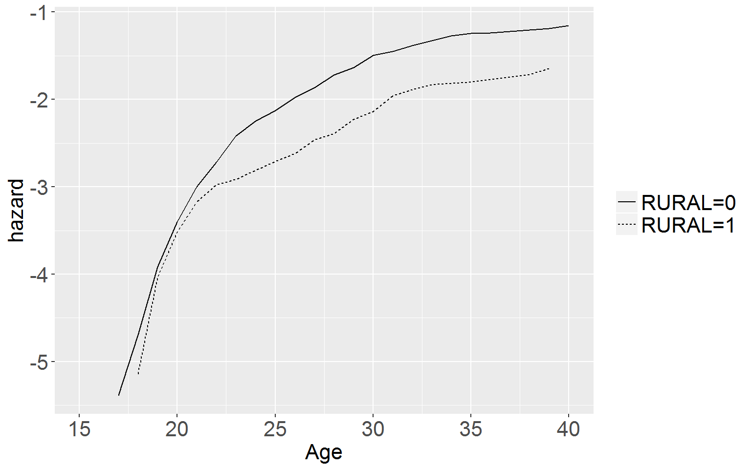
Table 15.3, p.560
Model C
For the first of the nonproportional hazards models we first we repeat model C from the first cocaine use analysis (see above) as a comparison model.
cocaineC <- read.csv("https://stats.idre.ucla.edu/stat/examples/alda/firstcocaine.csv")
cocaineC$EVENT <- 1 - cocaineC$CENSOR
cocaineC <- cocaineC[, c("ID", "COKEAGE", "EVENT", "MJAGE",
                         "ODAGE", "SELLMJAGE", "SDAGE", "BIRTHYR", "RURAL")]
dfC <- tmerge(cocaineC, cocaineC,
              id = ID,
              start_using = event(COKEAGE, EVENT),
              USEMJ = tdc(MJAGE),
              USEOD = tdc(ODAGE),
              SELLMJ = tdc(SELLMJAGE),
              SELLOD = tdc(SDAGE))

modC <- coxph(Surv(tstart, tstop, start_using) ~ BIRTHYR + USEMJ +
                USEOD + SELLMJ + SELLOD, data = dfC, ties="efron")
summary(modC)
## Call:
## coxph(formula = Surv(tstart, tstop, start_using) ~ BIRTHYR +
## USEMJ + USEOD + SELLMJ + SELLOD, data = dfC, ties = "efron")
##
## n= 3312, number of events= 382
##
## coef exp(coef) se(coef) z Pr(>|z|)
## BIRTHYR 0.08493 1.08864 0.02183 3.890 1e-04 ***
## USEMJ 2.45920 11.69542 0.28357 8.672 < 2e-16 ***
## USEOD 1.25110 3.49419 0.15656 7.991 1.33e-15 ***
## SELLMJ 0.68989 1.99349 0.12263 5.626 1.84e-08 ***
## SELLOD 0.76037 2.13908 0.13066 5.819 5.91e-09 ***
## ---
## Signif. codes: 0 '***' 0.001 '**' 0.01 '*' 0.05 '.' 0.1 ' ' 1
##
## exp(coef) exp(-coef) lower .95 upper .95
## BIRTHYR 1.089 0.9186 1.043 1.136
## USEMJ 11.695 0.0855 6.709 20.389
## USEOD 3.494 0.2862 2.571 4.749
## SELLMJ 1.993 0.5016 1.568 2.535
## SELLOD 2.139 0.4675 1.656 2.763
##
## Concordance= 0.89 (se = 0.015 )
## Rsquare= 0.248 (max possible= 0.811 )
## Likelihood ratio test= 944.5 on 5 df, p=0
## Wald test = 594.2 on 5 df, p=0
## Score (logrank) test = 1592 on 5 df, p=0Stratified Model
For the model stratified by RURAL we use the strata() function in the coxph call.
stratMod <- coxph(Surv(tstart, tstop, start_using) ~ BIRTHYR + USEMJ +
                    USEOD + SELLMJ + SELLOD + strata(RURAL), data= dfC, ties="efron")
summary(stratMod)
## Call:
## coxph(formula = Surv(tstart, tstop, start_using) ~ BIRTHYR +
## USEMJ + USEOD + SELLMJ + SELLOD + strata(RURAL), data = dfC,
## ties = "efron")
##
## n= 3312, number of events= 382
##
## coef exp(coef) se(coef) z Pr(>|z|)
## BIRTHYR 0.08537 1.08912 0.02187 3.903 9.51e-05 ***
## USEMJ 2.45795 11.68079 0.28370 8.664 < 2e-16 ***
## USEOD 1.25193 3.49710 0.15665 7.992 1.33e-15 ***
## SELLMJ 0.68473 1.98323 0.12284 5.574 2.49e-08 ***
## SELLOD 0.74684 2.11032 0.13126 5.690 1.27e-08 ***
## ---
## Signif. codes: 0 '***' 0.001 '**' 0.01 '*' 0.05 '.' 0.1 ' ' 1
##
## exp(coef) exp(-coef) lower .95 upper .95
## BIRTHYR 1.089 0.91817 1.043 1.137
## USEMJ 11.681 0.08561 6.699 20.369
## USEOD 3.497 0.28595 2.573 4.754
## SELLMJ 1.983 0.50423 1.559 2.523
## SELLOD 2.110 0.47386 1.632 2.729
##
## Concordance= 0.886 (se = 0.017 )
## Rsquare= 0.244 (max possible= 0.792 )
## Likelihood ratio test= 928.3 on 5 df, p=0
## Wald test = 584 on 5 df, p=0
## Score (logrank) test = 1511 on 5 df, p=0Within-Strata Model: Non-Rural
The final two columns of table 15.3 present separate within-strata results for the cocaine initiation data. We achieve this by simply creating two data frames: one with only the participants from non rural areas, the other with only those participants from rural areas. Start with the non-rural participants. The procedure for splitting the dataset with the tmerge() function is the same as above.
cocaineNonRural <- read.csv("https://stats.idre.ucla.edu/stat/examples/alda/firstcocaine.csv")
cocaineNonRural <- cocaineNonRural[cocaineNonRural$RURAL == 0,]
cocaineNonRural$EVENT <- 1 - cocaineNonRural$CENSOR
cocaineNonRural <- cocaineNonRural[, c("ID", "COKEAGE", "EVENT", "MJAGE",
                                       "ODAGE", "SELLMJAGE", "SDAGE", "BIRTHYR", "RURAL")]
est_dfNR <- tmerge(cocaineNonRural, cocaineNonRural,
                   id = ID,
                   start_using = event(COKEAGE, EVENT),
                   USEMJ = tdc(MJAGE),
                   USEOD = tdc(ODAGE),
                   SELLMJ = tdc(SELLMJAGE),
                   SELLOD = tdc(SDAGE))

modNR <- coxph(Surv(tstart, tstop, start_using) ~ BIRTHYR + USEMJ +
                 USEOD + SELLMJ + SELLOD, data= est_dfNR, ties="efron")
summary(modNR)
## Call:
## coxph(formula = Surv(tstart, tstop, start_using) ~ BIRTHYR +
## USEMJ + USEOD + SELLMJ + SELLOD, data = est_dfNR, ties = "efron")
##
## n= 2691, number of events= 328
##
## coef exp(coef) se(coef) z Pr(>|z|)
## BIRTHYR 0.08127 1.08467 0.02358 3.447 0.000567 ***
## USEMJ 2.43696 11.43818 0.31545 7.725 1.12e-14 ***
## USEOD 1.27272 3.57055 0.17157 7.418 1.19e-13 ***
## SELLMJ 0.71514 2.04446 0.13127 5.448 5.10e-08 ***
## SELLOD 0.69249 1.99869 0.14102 4.911 9.08e-07 ***
## ---
## Signif. codes: 0 '***' 0.001 '**' 0.01 '*' 0.05 '.' 0.1 ' ' 1
##
## exp(coef) exp(-coef) lower .95 upper .95
## BIRTHYR 1.085 0.92194 1.036 1.136
## USEMJ 11.438 0.08743 6.164 21.226
## USEOD 3.571 0.28007 2.551 4.998
## SELLMJ 2.044 0.48913 1.581 2.644
## SELLOD 1.999 0.50033 1.516 2.635
##
## Concordance= 0.886 (se = 0.016 )
## Rsquare= 0.251 (max possible= 0.818 )
## Likelihood ratio test= 776.9 on 5 df, p=0
## Wald test = 481.8 on 5 df, p=0
## Score (logrank) test = 1245 on 5 df, p=0Within-Strata Model: Rural
Now do the same for the RURAL participants.
cocaineRural <- read.csv("https://stats.idre.ucla.edu/stat/examples/alda/firstcocaine.csv")
cocaineRural <- cocaineRural[cocaineRural$RURAL == 1,]
cocaineRural$EVENT <- 1 - cocaineRural$CENSOR
cocaineRural <- cocaineRural[, c("ID", "COKEAGE", "EVENT", "MJAGE",
                                 "ODAGE", "SELLMJAGE", "SDAGE", "BIRTHYR")]
est_dfR <- tmerge(cocaineRural, cocaineRural,
                  id = ID,
                  start_using = event(COKEAGE, EVENT),
                  USEMJ = tdc(MJAGE),
                  USEOD = tdc(ODAGE),
                  SELLMJ = tdc(SELLMJAGE),
                  SELLOD = tdc(SDAGE))

modR <- coxph(Surv(tstart, tstop, start_using) ~ BIRTHYR + USEMJ +
                USEOD + SELLMJ + SELLOD, data= est_dfR, ties="efron")
summary(modR)
## Call:
## coxph(formula = Surv(tstart, tstop, start_using) ~ BIRTHYR +
## USEMJ + USEOD + SELLMJ + SELLOD, data = est_dfR, ties = "efron")
##
## n= 621, number of events= 54
##
## coef exp(coef) se(coef) z Pr(>|z|)
## BIRTHYR 0.10977 1.11603 0.05843 1.879 0.060282 .
## USEMJ 2.51796 12.40323 0.64875 3.881 0.000104 ***
## USEOD 1.14564 3.14445 0.38426 2.981 0.002869 **
## SELLMJ 0.45416 1.57486 0.35295 1.287 0.198179
## SELLOD 1.10501 3.01927 0.35231 3.136 0.001710 **
## ---
## Signif. codes: 0 '***' 0.001 '**' 0.01 '*' 0.05 '.' 0.1 ' ' 1
##
## exp(coef) exp(-coef) lower .95 upper .95
## BIRTHYR 1.116 0.89604 0.9953 1.251
## USEMJ 12.403 0.08062 3.4779 44.234
## USEOD 3.144 0.31802 1.4807 6.678
## SELLMJ 1.575 0.63498 0.7885 3.145
## SELLOD 3.019 0.33121 1.5136 6.023
##
## Concordance= 0.897 (se = 0.04 )
## Rsquare= 0.218 (max possible= 0.628 )
## Likelihood ratio test= 153 on 5 df, p=0
## Wald test = 106 on 5 df, p=0
## Score (logrank) test = 324.4 on 5 df, p=0To conduct a formal test of the null hypothesis that within-strata parameters are identical across strata, and identical to their counterparts in the model itself, you simply compare the -2LL statistics for separate models fitted within each stratum. In our example we calculate the test statistic by subtracting the sum of the -2LL statistics for the two within-strata models from the deviance statistic of the stratified model.
devNonRural <- -2*logLik(modNR)
devRural <- -2*logLik(modR)
devStratMod <- -2*logLik(stratMod)
diff <- devStratMod - (devRural + devNonRural)
diff
## 'log Lik.' 1.584091 (df=5)To test the null hypothesis that the set of parameters is identical across the strata. Compare this value to the critical cutoff of p <.05 a chi-square distribution with 5 d.f.
qchisq(.95,5)## [1] 11.07051.584 < 11.08, therefore we cannot reject the null that the parameters are identical across strata, which means that the stratified model is probably suitable.
Table 15.4 p.566
Model A
Read in data.
los <- read.csv("https://stats.idre.ucla.edu/stat/examples/alda/lengthofstay.csv")Note: there is a duplicate id number in this dataset. So we have to change it to a new ID number.
los$ID[which(duplicated(los$ID))] <- 842Next make an event variable.
los$EVENT <- 1 - los$CENSORNow fit model A.
modA <- coxph(Surv(DAYS,EVENT) ~ TREAT, data = los)
summary(modA)
## Call:
## coxph(formula = Surv(DAYS, EVENT) ~ TREAT, data = los)
##
## n= 174, number of events= 172
##
## coef exp(coef) se(coef) z Pr(>|z|)
## TREAT 0.1457 1.1568 0.1541 0.945 0.345
##
## exp(coef) exp(-coef) lower .95 upper .95
## TREAT 1.157 0.8644 0.8552 1.565
##
## Concordance= 0.554 (se = 0.023 )
## Rsquare= 0.005 (max possible= 1 )
## Likelihood ratio test= 0.89 on 1 df, p=0.3449
## Wald test = 0.89 on 1 df, p=0.3446
## Score (logrank) test = 0.89 on 1 df, p=0.3442Model B
For model B We need to create a person-period, count-process dataset. Again we use the survSplit() function. First we make a vector of all the time points when an event occurred and split the dataset using that vector.
cutPoints <- sort(unique(los$DAYS[los$EVENT == 1]))
longLOS <- survSplit(Surv(DAYS,EVENT)~.,
                     data = los,
                     cut = cutPoints,
                     end = "tstop")
Next we create the interaction variable.
longLOS$TREATINT <- longLOS$TREAT*(longLOS$tstop - 1)Then fit the model.
modB <- coxph(Surv(tstart, tstop, EVENT) ~ TREAT + TREATINT, data = longLOS)
summary(modB)
## Call:
## coxph(formula = Surv(tstart, tstop, EVENT) ~ TREAT + TREATINT,
## data = longLOS)
##
## n= 3991, number of events= 172
##
## coef exp(coef) se(coef) z Pr(>|z|)
## TREAT 0.706411 2.026705 0.292404 2.416 0.0157 *
## TREATINT -0.020833 0.979383 0.009207 -2.263 0.0237 *
## ---
## Signif. codes: 0 '***' 0.001 '**' 0.01 '*' 0.05 '.' 0.1 ' ' 1
##
## exp(coef) exp(-coef) lower .95 upper .95
## TREAT 2.0267 0.4934 1.1426 3.5949
## TREATINT 0.9794 1.0211 0.9619 0.9972
##
## Concordance= 0.557 (se = 0.023 )
## Rsquare= 0.002 (max possible= 0.302 )
## Likelihood ratio test= 6.15 on 2 df, p=0.04628
## Wald test = 6 on 2 df, p=0.0499
## Score (logrank) test = 6.18 on 2 df, p=0.04561We can test the difference in -2LL statistic from Model A using a likelihood ratio test.
(-2*logLik(modA) - -2*logLik(modB))## 'log Lik.' 5.253742 (df=1)When we compare this to the critical value for a \(\chi^2\) distribution on 1 d.f…..
qchisq(.95,1)## [1] 3.8414595.25 is greater than the critical value of 3.84, therefore model B is a significantly better fit than model A (p < .05).
Model C
Model C uses a piecewise specification of time. To do this we define six weekly time periods, the first representing days 0-7, the intermediate periods representing 8-14, 15-21, 22-28, and 29-35 days , and the final period representing days 36 on. These divisions were based on examination of figure 15.3, the declining number of events during the later days, and an examination of parameter estimates from finer classifications.
First we split the dataset on the epochs discussed above, using the cut() and episode() arguments in survSplit(). The values input here are the END times for each of the epochs.
longLOS2 <- survSplit(Surv(DAYS,EVENT)~.,
                      data = los,
                      end = "tstop",
                      cut = c(7,14,21,28,35),
                      episode = "epoch",
                      id = "id")
Now fit the model.
modC <- coxph(Surv(tstart, tstop, EVENT) ~ TREAT:strata(epoch), data=longLOS2)
summary(modC)
## Call:
## coxph(formula = Surv(tstart, tstop, EVENT) ~ TREAT:strata(epoch),
## data = longLOS2)
##
## n= 695, number of events= 172
##
## coef exp(coef) se(coef) z Pr(>|z|)
## TREAT:strata(epoch)epoch=1 1.57114 4.81212 0.64061 2.453 0.0142 *
## TREAT:strata(epoch)epoch=2 0.56779 1.76436 0.49285 1.152 0.2493
## TREAT:strata(epoch)epoch=3 0.84970 2.33896 0.36207 2.347 0.0189 *
## TREAT:strata(epoch)epoch=4 -0.34986 0.70479 0.36415 -0.961 0.3367
## TREAT:strata(epoch)epoch=5 -0.76969 0.46316 0.41598 -1.850 0.0643 .
## TREAT:strata(epoch)epoch=6 -0.06906 0.93327 0.31447 -0.220 0.8262
## ---
## Signif. codes: 0 '***' 0.001 '**' 0.01 '*' 0.05 '.' 0.1 ' ' 1
##
## exp(coef) exp(-coef) lower .95 upper .95
## TREAT:strata(epoch)epoch=1 4.8121 0.2078 1.3710 16.890
## TREAT:strata(epoch)epoch=2 1.7644 0.5668 0.6715 4.636
## TREAT:strata(epoch)epoch=3 2.3390 0.4275 1.1503 4.756
## TREAT:strata(epoch)epoch=4 0.7048 1.4189 0.3452 1.439
## TREAT:strata(epoch)epoch=5 0.4632 2.1591 0.2049 1.047
## TREAT:strata(epoch)epoch=6 0.9333 1.0715 0.5039 1.729
##
## Concordance= 0.591 (se = 0.052 )
## Rsquare= 0.028 (max possible= 0.874 )
## Likelihood ratio test= 19.74 on 6 df, p=0.003085
## Wald test = 17.24 on 6 df, p=0.008425
## Score (logrank) test = 19.14 on 6 df, p=0.003931Now calculate difference in -2LL statistics for Model A and Model C and compare this difference to the critical values of a \(\chi^2\) distribution with 6 – 1 = 5 degrees of freedom.
abs(-2*logLik(modC) - -2*logLik(modA)); qchisq(.99,5)## 'log Lik.' 18.84432 (df=6)## [1] 15.0862718.84 > 15.09, therefore we can reject null and conclude Model C is an improvement on Model A.
Model D
For Model D we use the survSplit function once again, but cutting by all event times rather than the epochs we used in Model C
cutPoints <- sort(unique(los$DAYS[los$EVENT == 1]))
longLOS3 <- survSplit(Surv(DAYS,EVENT)~.,
                      data = los,
                      cut = cutPoints,
                      end = "tstop")
Next we create the interaction variable. Because log(0) = \(\infty\) we need to add a small constant to any 0 values in the tstop variable,
longLOS3$TREATINT <- longLOS3$TREAT*log2(longLOS3$tstop + .001)Now fit the model
modD <- coxph(Surv(tstart, tstop, EVENT) ~ TREAT + TREATINT, data=longLOS3)
summary(modD)
## Call:
## coxph(formula = Surv(tstart, tstop, EVENT) ~ TREAT + TREATINT,
## data = longLOS3)
##
## n= 3991, number of events= 172
##
## coef exp(coef) se(coef) z Pr(>|z|)
## TREAT 2.5338 12.6007 0.7604 3.332 0.000862 ***
## TREATINT -0.5302 0.5885 0.1619 -3.275 0.001058 **
## ---
## Signif. codes: 0 '***' 0.001 '**' 0.01 '*' 0.05 '.' 0.1 ' ' 1
##
## exp(coef) exp(-coef) lower .95 upper .95
## TREAT 12.6007 0.07936 2.8389 55.9287
## TREATINT 0.5885 1.69921 0.4285 0.8083
##
## Concordance= 0.584 (se = 0.023 )
## Rsquare= 0.004 (max possible= 0.302 )
## Likelihood ratio test= 14.46 on 2 df, p=0.0007254
## Wald test = 11.11 on 2 df, p=0.00387
## Score (logrank) test = 13.2 on 2 df, p=0.001358Once again let’s calculate the difference in -2LL statistics between Models D and compare this to the critical difference on a \(\chi^2\) distribution with 2-1 = 1 degrees of freedom.
abs(-2*logLik(modD) - -2*logLik(modA))## 'log Lik.' 13.5653 (df=2)qchisq(.999,1)## [1] 10.82757Based on the difference in -2LL statistics being greater than the critical value, we can reject null at the p = .001 level, concluding that Model D is superior to Model A.
Fig 15.3 p.567
Top Panel
First we construct the life table, split by TREAT
t15.3a <- summary(losLife <- survfit(Surv(DAYS, EVENT)~TREAT, data = los))

# turn it into a df
df15.3a <- data.frame(group = t15.3a$strata,
                      time = t15.3a$time,
                      event = t15.3a$n.event,
                      risk = t15.3a$n.risk,
                      censored = t15.3a$n.censor,
                      survival = t15.3a$surv,
                      se = t15.3a$std.err,
                      hazard = t15.3a$n.event/t15.3a$n.risk)

# now create the width variable
for (i in 1:nrow(df15.3a)){
  df15.3a[i,"width"] <- df15.3a[i+1,"time"] - df15.3a[i,"time"]
}

# now add kaplan-meier hazard and neg log cumulative hazard
df15.3a$hKM <-  df15.3a$hazard/df15.3a$width
df15.3a$negLogCumHaz <- -log(df15.3a$survival)

# now add the log cumulative hazard function, which we do by logging the neg log cumulative hazard values
df15.3a$logHaz <- log(df15.3a$negLogCumHaz)

# add the first row
df15.3a <- rbind(c("TREAT=0", 0, 0, t15.3a$n[1], 0, 1, 0, 0, 0, 0, 0, NA), df15.3a)

# make everything numeric
for (i in 2:length(df15.3a)) { df15.3a[,i] <- as.numeric(df15.3a[,i]) }

# now graph the cumulative log hazard function
ggplot(df15.3a, aes(x = time, y = logHaz, linetype = group)) +
       geom_line() +
       coord_cartesian(xlim = c(7,77)) +
       scale_x_continuous(breaks = seq(0,77,7)) +
       xlab("Days in Treatment") + ylab("hazard") +
       theme(legend.text = element_text(size = 16),
             legend.title = element_blank(),
             axis.title.x = element_text(size = 16),
             axis.title.y = element_text(size = 16),
             axis.text.x = element_text(size = 16),
             axis.text.y = element_text(size = 16))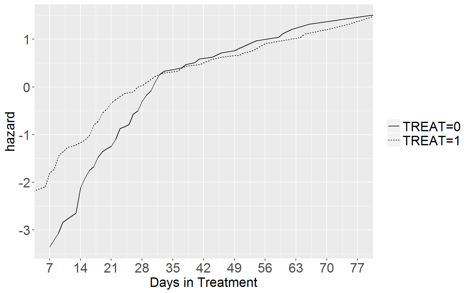
Lower Panel
# split df15.3a
df15.3b_treat0 <- df15.3a[df15.3a$group == "TREAT=0", c("time", "logHaz")]
names(df15.3b_treat0)[2] <- "logCumHaz0"
df15.3b_treat1 <- df15.3a[df15.3a$group == "TREAT=1", c("time", "logHaz")]
names(df15.3b_treat1)[2] <- "logCumHaz1"

# now merge the two datasets. This will 'edit out' the event time points the two groups do not share
df15.3b_merge <- merge(df15.3b_treat0, df15.3b_treat1, "time")

# get the difference in log cumulative hazard
df15.3b_merge$diff <- df15.3b_merge$logCumHaz1 - df15.3b_merge$logCumHaz0

# restrict the time frame we look at
df15.3b_merge <- df15.3b_merge[df15.3b_merge$time < 61,]

# now plot
ggplot(df15.3b_merge, aes(y = diff, x = time)) +
      geom_line() +
      geom_hline(yintercept = 0, linetype = 3) +
      coord_cartesian(xlim = c(0,77)) +
      scale_x_continuous(breaks = seq(0,77,7)) +
      xlab("Days in Treatment") + ylab("difference in hazard") +
      theme(legend.text = element_text(size = 16),
            legend.title = element_blank(),
            axis.title.x = element_text(size = 16),
            axis.title.y = element_text(size = 16),
            axis.text.x = element_text(size = 16),
            axis.text.y = element_text(size = 16))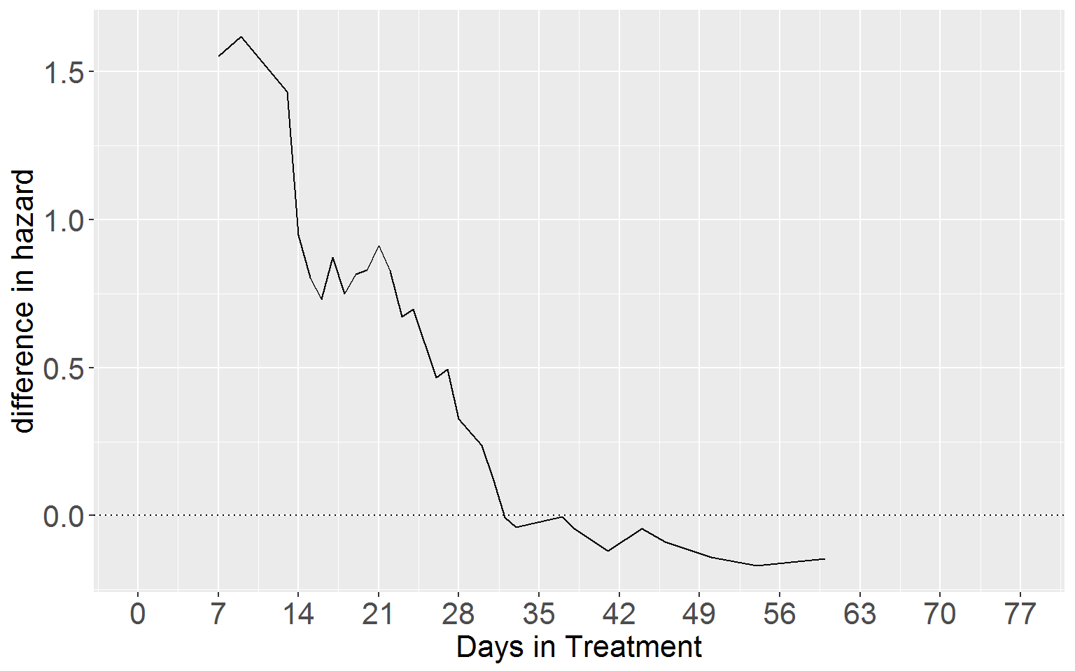
Figure 15.4 p.573
R has excellent residuals functions and the coxph() function is no exception.
rearrest <- read.csv("https://stats.idre.ucla.edu/stat/examples/alda/rearrest.csv")

# the null model
nullSum <- summary(nullMod <- coxph(Surv(months, 1 - censor)~1, data = rearrest))

# model D, with all predictors entered into the model at once
fullSum <- summary(fullMod <- coxph(Surv(months, 1 - censor)~personal + property + cage,
                                    data = rearrest))

# martingale residuals

# attach the martingale residuals to the data set.
rearrest$residMart_null <- resid(nullMod, type = "martingale")
rearrest$residMart_full <- resid(fullMod, type = "martingale")
Top Panel
Now we plot the martingale residuals from the null model against AGE with a loess smooth. Use the span() argument within geom_smooth() to adjust the ‘wiggliness’ of the smooth.
 ggplot(rearrest, aes(x = cage, y = residMart_null)) +
        geom_point(aes(shape = factor(censor)), size = 3.5) +
        geom_smooth(stat = "smooth", method = "loess", se = FALSE, span = 1) +
        xlab("AGE") + ylab("martingale residuals - null model") +
        scale_shape_manual(values = c(16,3)) +
        geom_hline(yintercept = 0, linetype = "dashed", size = 0.25) +
        coord_cartesian(ylim=c(-3,1)) +
        theme(legend.position = "none",
              axis.title.x = element_text(size = 16),
              axis.title.y = element_text(size = 16),
              axis.text.x = element_text(size = 16),
              axis.text.y = element_text(size = 16))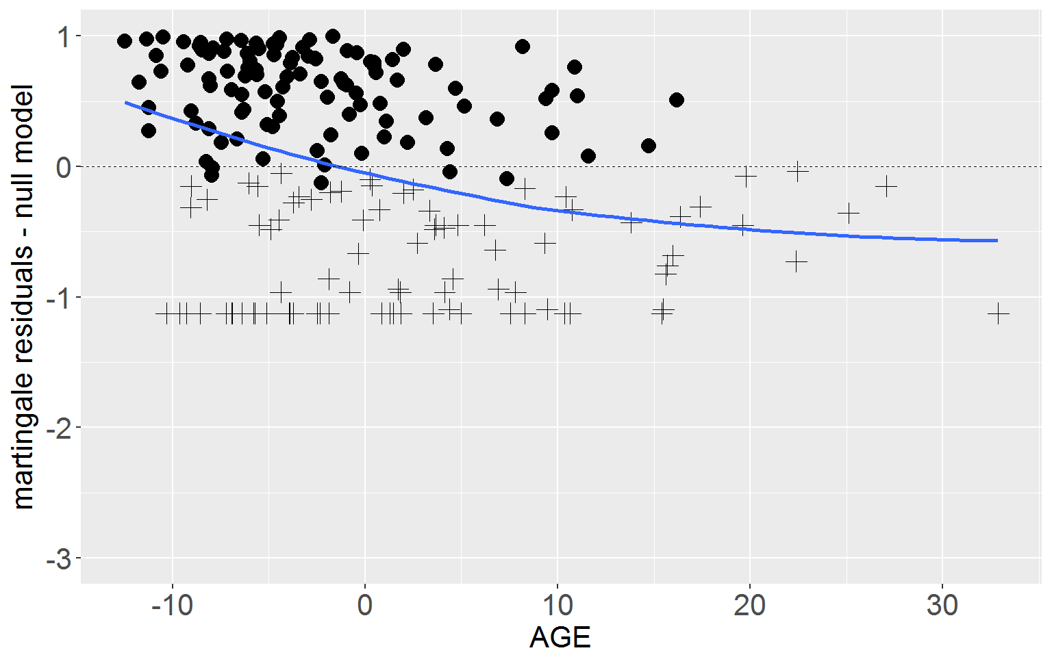
Lower Panel
Next plot the martingale residuals from the full model against AGE.
 ggplot(rearrest, aes(x = cage, y = residMart_full)) +
        geom_point(aes(shape = factor(censor)), size = 3.5) +
        geom_smooth(stat = "smooth", method = "loess", se = FALSE, span = 1) +
        xlab("AGE") + ylab("martingale residuals - full model") +
        scale_shape_manual(values = c(16,3)) +
        geom_hline(yintercept = 0, linetype = "dashed", size = 0.25) +
        coord_cartesian(ylim=c(-3,1)) +
        theme(legend.position = "none",
              axis.title.x = element_text(size = 16),
              axis.title.y = element_text(size = 16),
              axis.text.x = element_text(size = 16),
              axis.text.y = element_text(size = 16))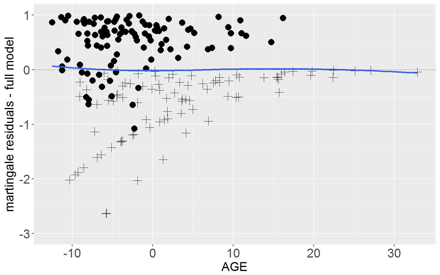
Figure 15.5 p.577
Stem and Leaf Plot
First attach the deviance residuals to the dataset.
rearrest$residDev <- resid(fullMod, type = "deviance")Now we can the stem and leaf plot. We specify scale = 2 to get the right scale for this display. The order of the values is the exac reverse of to those in the book, but the distribution is exactly the same.
stem(rearrest$residDev, scale = 2)##
## The decimal point is 1 digit(s) to the left of the |
##
## -22 | 09
## -20 | 21
## -18 | 6491
## -16 | 969321
## -14 | 54216
## -12 | 87654741
## -10 | 208776542110
## -8 | 99852176544
## -6 | 876322098874400
## -4 | 444443332877644210
## -2 | 85009955411
## -0 | 997597551
## 0 | 268979
## 2 | 0318
## 4 | 133678802337
## 6 | 2688919
## 8 | 1136690012233889999
## 10 | 122334724789
## 12 | 0115
## 14 | 0228055578
## 16 | 03795
## 18 | 2336
## 20 | 0735
## 22 | 6
## 24 | 00
## 26 | 7Plot Deviance Residuals
We need to calculate risk scores for each individual (the predicted log hazard based on the model coefficients and each individual’s values for the predictors).
rearrest$riskScore <- coef(fullMod)[1]*rearrest$personal +
  coef(fullMod)[2]*rearrest$property +
  coef(fullMod)[3]*rearrest$cage
Now we can plot residuals against log risk score.
 ggplot(rearrest, aes(x = riskScore, y = residDev)) +
        geom_point(aes(shape = factor(censor)), size = 3.5) +
        xlab("risk score") + ylab("deviance residuals") +
        scale_shape_manual(values = c(16,3)) +
        geom_hline(yintercept = 0, linetype = "dashed", size = 0.25) +
        coord_cartesian(xlim = c(-3,3), ylim = c(-3,3)) +
        scale_y_continuous(breaks = seq(-3,3,1)) +
        scale_x_continuous(breaks = seq(-3,3,1)) +
        theme(legend.position = "none",
              axis.title.x = element_text(size = 16),
              axis.title.y = element_text(size = 16),
              axis.text.x = element_text(size = 16),
              axis.text.y = element_text(size = 16))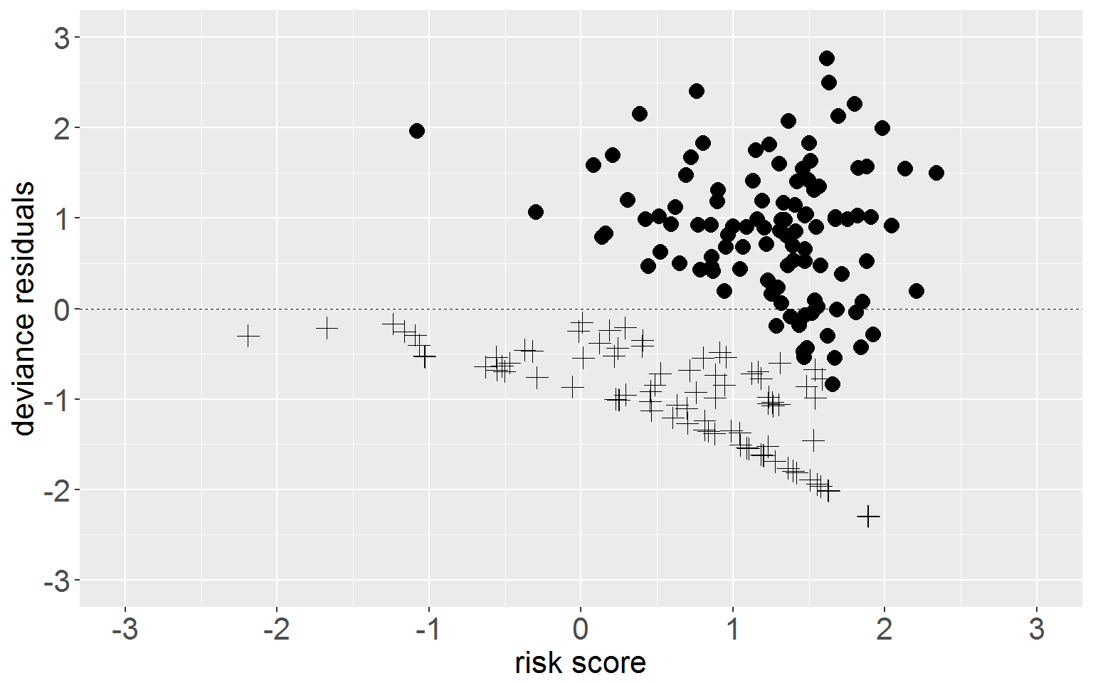
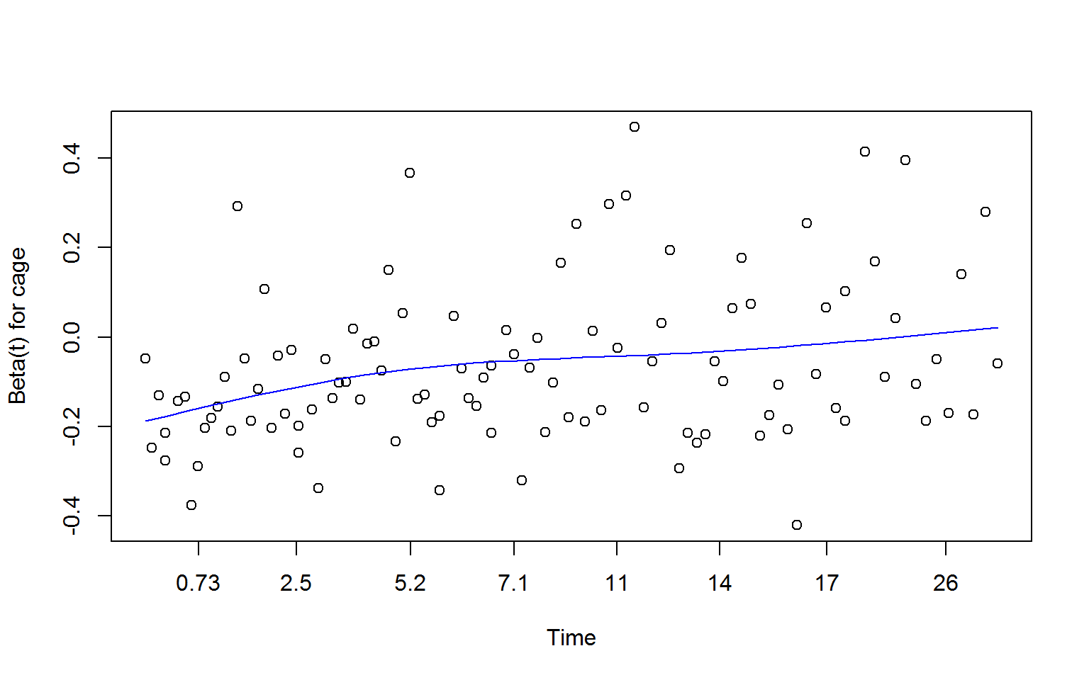
Figure 15.6 p.580
You can plot Schoenfeld residuals in at least two ways, first with the cox.zph() and native plot() functions, secondly with resid() and ggplot()
cox.zph() Method
zSchoen <- cox.zph(fullMod)
plot(zSchoen, se = FALSE, col = "blue") # will produce three plots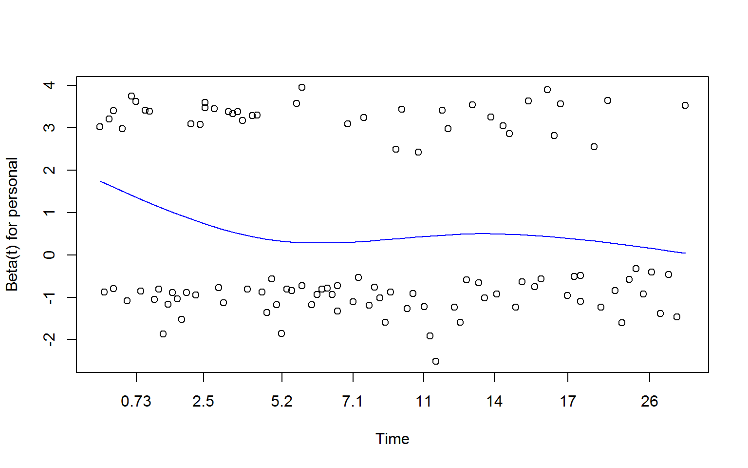
resid() and ggplot() Method
First we attach the Schoenfeld residuals to our dataset.
schoen <- resid(fullMod, type = "schoenfeld")Next assign a rank for each event time.
rearrest$rankTime <- rank(rearrest$months, ties.method = "average") # rank timeSchoenfeld residuals only pertain to those who experience the event (here 106), so if we are going to bind the residuals to the dataset we need to reduce the dataset to the number of people who experienced the event (note here censor = 0 indicates someone who experienced the event).
rearrestEvent <- dplyr::filter(rearrest, censor == 0)Now let’s get the residuals for each of the predictors by separating them from the 3 x 10⁶ matrix and binding each to the reduced dataset
rearrestEvent$schoenPers <- schoen[,1]
rearrestEvent$schoenProp <- schoen[,2]
rearrestEvent$schoenAge <- schoen[,3]
Next we need to calculate the correlation coefficients between rank time and each of the Schoenfeld residuals columns.
persCorr <- cor.test(rearrestEvent$rankTime, rearrestEvent$schoenPers, method = "pearson")
propCorr <- cor.test(rearrestEvent$rankTime, rearrestEvent$schoenProp, method = "pearson")
ageCorr <- cor.test(rearrestEvent$rankTime, rearrestEvent$schoenAge, method = "pearson")
Personal
Now we can plot Schoenfeld residuals for personal crime against rank time.
 ggplot(rearrestEvent, aes(x = rankTime, y = schoenPers)) +
        geom_point(aes(shape = factor(censor)), size = 3.5) +
        geom_smooth(stat = "smooth", method = "loess", span = 1, se = FALSE) +
        xlab("Rank (months)") + ylab("schoenfeld residuals - personal") +
        scale_shape_manual(values = c(16,3)) +
        geom_hline(yintercept = 0, linetype = "dashed", size = 0.25) +
        coord_cartesian(ylim = c(-.5,1), xlim = c(0,175)) +
        scale_y_continuous(breaks = seq(-.5,1,.5)) +
        scale_x_continuous(breaks = seq(0,175,25)) +
        theme(legend.position = "none",
              axis.title.x = element_text(size = 16),
              axis.title.y = element_text(size = 16),
              axis.text.x = element_text(size = 16),
              axis.text.y = element_text(size = 16)) +
        annotate("text", x = 150, y = 0.3,
                 label = paste("r =",
                               format(round(persCorr$estimate,2), nsmall = 2),
                               ", p = ",
                               format(round(persCorr$p.value,2), nsmall = 2),
                               sep = ""),
                 size = 5)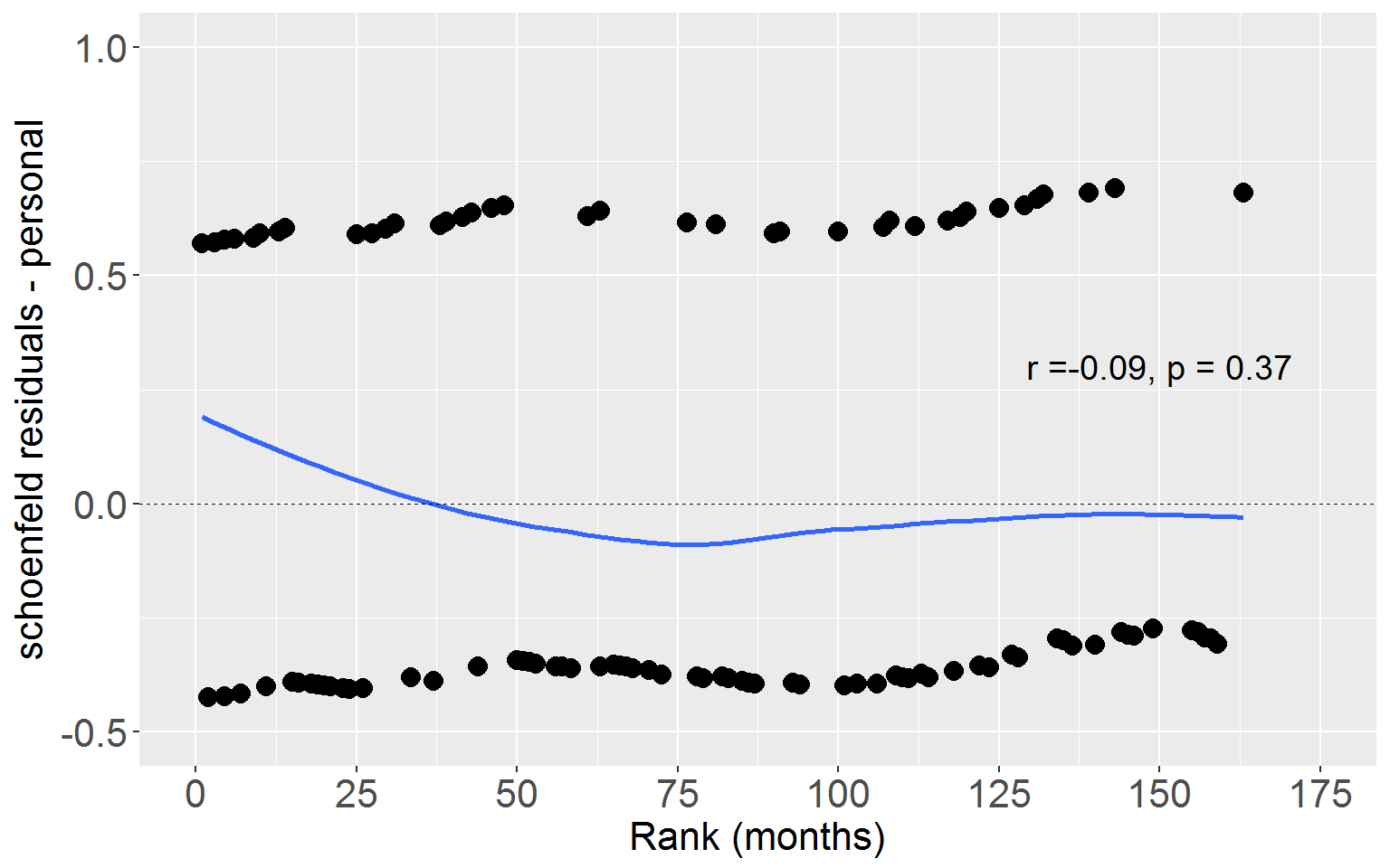
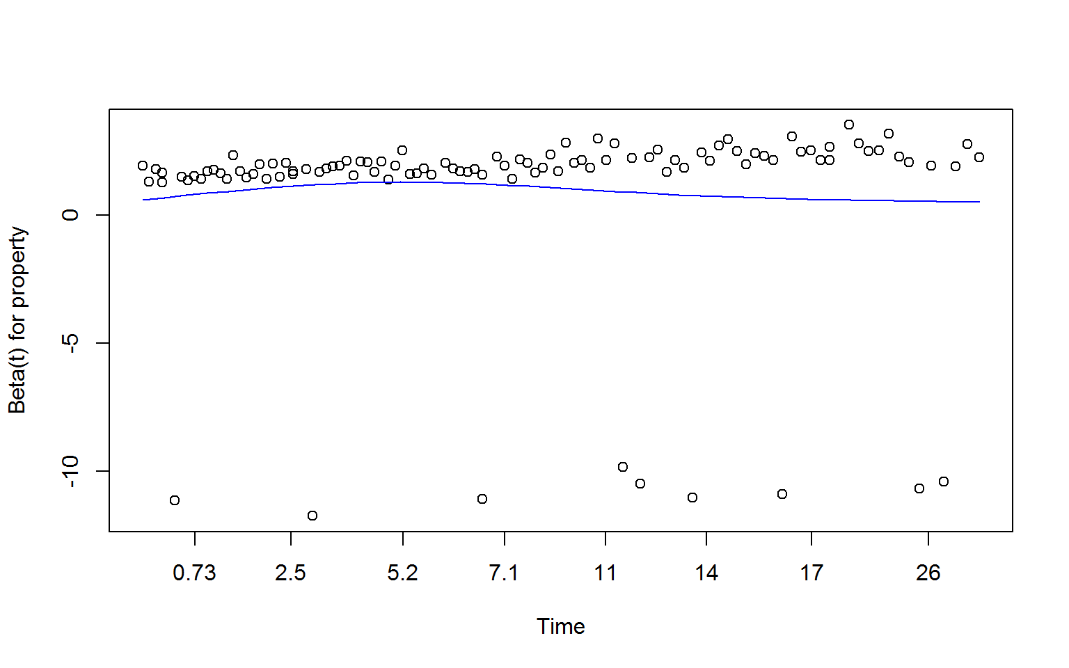
Property
Next plot Schoenfeld residuals for property crime against rank time.
 ggplot(rearrestEvent, aes(x = rankTime, y = schoenProp)) +
        geom_point(aes(shape = factor(censor)), size = 3.5) +
        geom_smooth(stat = "smooth", method = "loess", span = 1, se = FALSE) +
        xlab("Rank (months)") + ylab("schoenfeld residuals - property") +
        scale_shape_manual(values = c(16,3)) +
        geom_hline(yintercept = 0, linetype = "dashed", size = 0.25) +
        coord_cartesian(ylim = c(-1,.2), xlim = c(0,175)) +
        scale_y_continuous(breaks = seq(-1,.2,.2)) +
        scale_x_continuous(breaks = seq(0,175,25)) +
        theme(legend.position = "none",
              axis.title.x = element_text(size = 16),
              axis.title.y = element_text(size = 16),
              axis.text.x = element_text(size = 16),
              axis.text.y = element_text(size = 16)) +
        annotate("text", x = 150, y = -0.3,
                 label = paste("r =",
                               format(round(propCorr$estimate,2), nsmall = 2),
                               ", p = ",
                               format(round(propCorr$p.value,2), nsmall = 2),
                               sep = ""),
                 size = 5)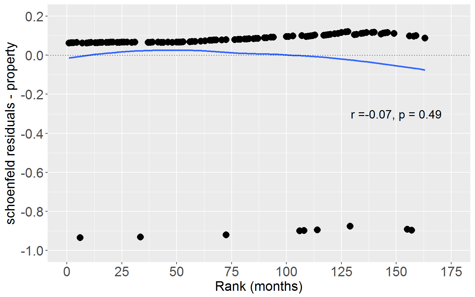
Age
Lastly plot Schoenfeld residuals for age against rank time.
 ggplot(rearrestEvent, aes(x = rankTime, y = schoenAge)) +
        geom_point(aes(shape = factor(censor)), size = 3.5) +
        geom_smooth(stat = "smooth", method = "loess", span = 1, se = FALSE) +
        xlab("Rank (months)") + ylab("schoenfeld residuals - age") +
        scale_shape_manual(values = c(16,3)) +
        geom_hline(yintercept = 0, linetype = "dashed", size = 0.25) +
        coord_cartesian(ylim = c(-10,20), xlim = c(0,175)) +
        scale_y_continuous(breaks = seq(-10,20,10)) +
        scale_x_continuous(breaks = seq(0,175,25)) +
        theme(legend.position = "none",
              axis.title.x = element_text(size = 16),
              axis.title.y = element_text(size = 16),
              axis.text.x = element_text(size = 16),
              axis.text.y = element_text(size = 16)) +
        annotate("text", x = 25, y = 18,
                 label = paste("r =",
                               format(round(ageCorr$estimate,2), nsmall = 2),
                               ", p = ",
                               format(round(ageCorr$p.value,2), nsmall = 2),
                               sep = ""),
                 size = 5)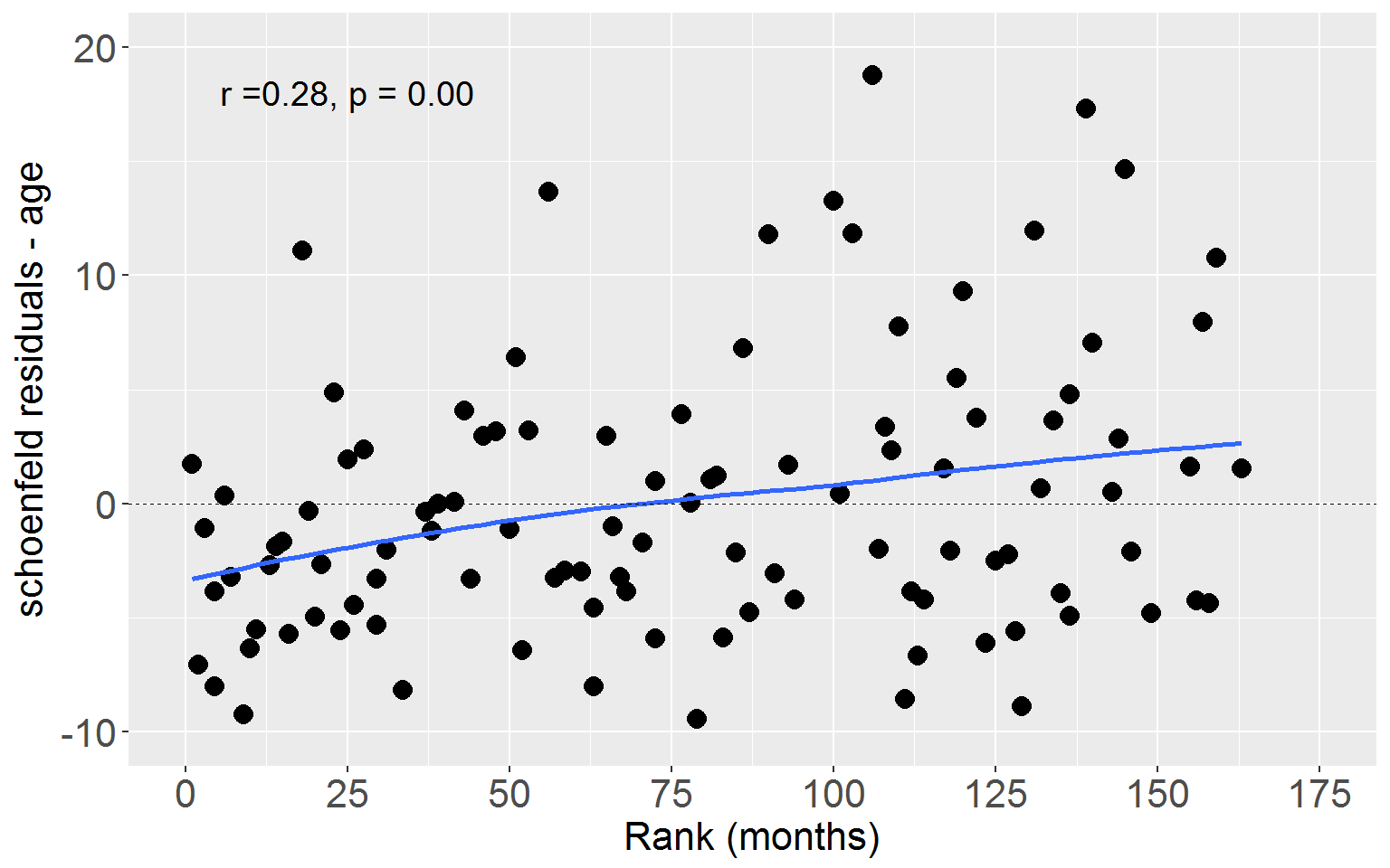
Figure 15.7 p.583
Attach score residuals to the rearrest dataset
scoreResid <- resid(fullMod, type = "score")

rearrest$residScorePers <- scoreResid[,1]
rearrest$residScoreProp <- scoreResid[,2]
rearrest$residScoreAge  <- scoreResid[,3]
Now we plot the score residuals against the log risk score.
Personal
 ggplot(rearrest, aes(x = rankTime, y = residScorePers)) +
        geom_point(aes(shape = factor(censor)), size = 3.5) +
        xlab("Rank (months)") + ylab("Personal") +
        scale_shape_manual(values = c(16,3)) +
        geom_hline(yintercept = 0, linetype = "dashed", size = 0.25) +
        coord_cartesian(xlim = c(0,175), ylim = c(-2,1)) +
        scale_y_continuous(breaks = seq(-2,1,1)) +
        scale_x_continuous(breaks = seq(0,175,25)) +
        theme(legend.position = "none",
              axis.title.x = element_text(size = 16),
              axis.title.y = element_text(size = 16),
              axis.text.x = element_text(size = 16),
              axis.text.y = element_text(size = 16))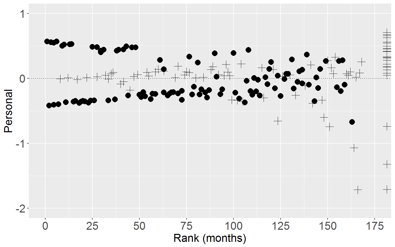
Personal
 ggplot(rearrest, aes(x = rankTime, y = residScoreProp)) +
        geom_point(aes(shape = factor(censor)), size = 3.5) +
        xlab("Rank (months)") + ylab("Property") +
        scale_shape_manual(values = c(16,3)) +
        geom_hline(yintercept = 0, linetype = "dashed", size = 0.25) +
        coord_cartesian(xlim = c(0,175), ylim = c(-1,1.2)) +
        scale_y_continuous(breaks = seq(-1,1.2,.4)) +
        scale_x_continuous(breaks = seq(0,175,25)) +
        theme(legend.position = "none",
              axis.title.x = element_text(size = 16),
              axis.title.y = element_text(size = 16),
              axis.text.x = element_text(size = 16),
              axis.text.y = element_text(size = 16))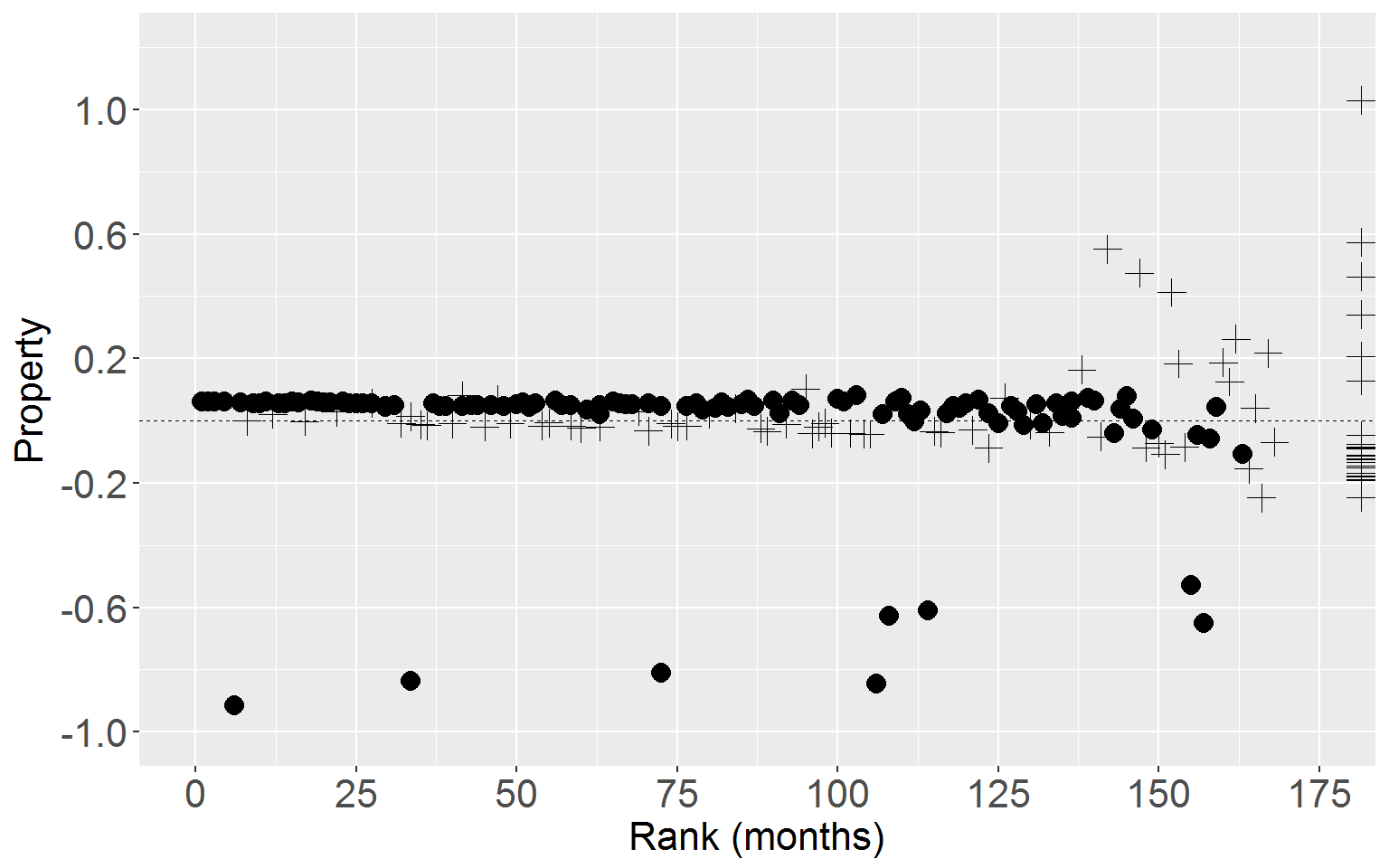
Age
 ggplot(rearrest, aes(x = rankTime, y = residScoreAge)) +
        geom_point(aes(shape = factor(censor)), size = 3.5) +
        xlab("Rank (months)") + ylab("Age") +
        scale_shape_manual(values = c(16,3)) +
        geom_hline(yintercept = 0, linetype = "dashed", size = 0.25) +
        coord_cartesian(xlim = c(0,175), ylim = c(-10,20)) +
        scale_y_continuous(breaks = seq(-10,20,10)) +
        scale_x_continuous(breaks = seq(0,175,25)) +
        theme(legend.position = "none",
              axis.title.x = element_text(size = 16),
              axis.title.y = element_text(size = 16),
              axis.text.x = element_text(size = 16),
              axis.text.y = element_text(size = 16))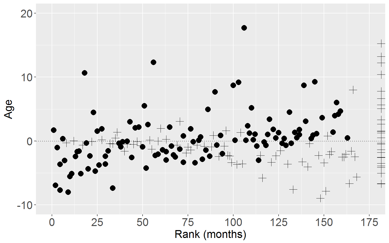
Figure 15.8 p.589
First we need to prepare the life table for the judges dataset.
# read in the dataset
judges <- read.csv("https://stats.idre.ucla.edu/stat/examples/alda/judges.csv")

# create the two life table objects
jSum_retire <- summary(survfit(Surv(judges$tenure, judges$retire)~1))
jSum_die <- summary(survfit(Surv(judges$tenure, judges$dead)~1))

# now to graph these we need to bind the two together.
# the `survfit()` object is not a data.frmae nor can it be coerced to be one,
# so we extract the relevant information.

# first the 'retire' life table
jsRetireDF <- data.frame(time = jSum_retire$time,
                         n.risk = jSum_retire$n.risk,
                         n.event = jSum_retire$n.event,
                         n.censor = jSum_retire$n.censor,
                         surv = jSum_retire$surv,
                         se = jSum_retire$std.err,
                         hazard = jSum_retire$n.risk/jSum_retire$n.event,
                         group = 0) # put a group signifier in

# add width variable
for (i in 1:nrow(jsRetireDF)){
  jsRetireDF[i,"width"] <- jsRetireDF[i+1,"time"] - jsRetireDF[i,"time"]
}

# add kaplan meier and neg log cumulative hazard function
jsRetireDF$hKM = jsRetireDF$hazard/jsRetireDF$width
jsRetireDF$negLogCumHaz <- -log(jsRetireDF$surv)
jsRetireDF$logHaz = log(jsRetireDF$negLogCumHaz)

# create top row
jsRetireDF <- rbind(c(0,109,0,0,1,0,0,0,0,0,0,0),jsRetireDF) # make the first row

# now the 'die' dataset
jsDieDF <- data.frame(time = jSum_die$time,
                      n.risk = jSum_die$n.risk,
                      n.event = jSum_die$n.event,
                      n.censor = jSum_die$n.censor,
                      surv = jSum_die$surv,
                      se = jSum_die$std.err,
                      hazard = jSum_die$n.risk/jSum_die$n.event,
                      group = 1) # group signifier

# add width variable
for (i in 1:nrow(jsDieDF)){
  jsDieDF[i,"width"] <- jsDieDF[i+1,"time"] - jsDieDF[i,"time"]
}

# add kaplan meier, neg log cumulative hazard function, and cumulative hazard function
jsDieDF$hKM <- jsDieDF$hazard/jsDieDF$width
jsDieDF$negLogCumHaz = -log(jsDieDF$surv)
jsDieDF$logHaz = log(jsDieDF$negLogCumHaz)

# add first row
jsDieDF <- rbind(c(0,106,0,0,1,0,0,1,0,0,0,0),jsDieDF) # make the first row

# bind the two life tables together
judgesLT <- rbind(jsRetireDF, jsDieDF)

# add labels
judgesLT$group <- factor(judgesLT$group, levels = 0:1, labels = c("retire", "die"))
Survivor Function
 ggplot(judgesLT, aes(x = time, y = surv, group = group)) +
        geom_step(aes(linetype = group)) +
        xlab("years on court") + ylab("survival") +
        coord_cartesian(xlim = c(0,35)) +
        scale_x_continuous(breaks = seq(0,35,5)) +
        theme(legend.text = element_text(size = 16),
              legend.title = element_blank(),
              axis.title.x = element_text(size = 16),
              axis.title.y = element_text(size = 16),
              axis.text.x = element_text(size = 16),
              axis.text.y = element_text(size = 16))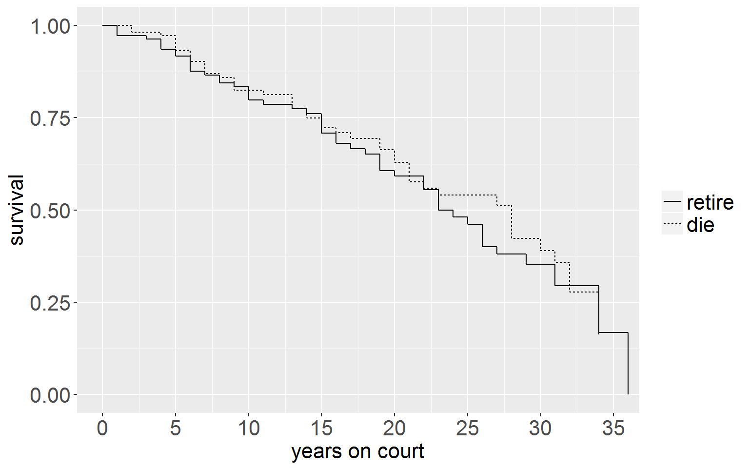
Log Cumulative Hazard Function
 ggplot(judgesLT, aes(x = time, y = negLogCumHaz, group = group)) +
        geom_step(aes(linetype = group)) +
        xlab("years on court") + ylab("cumulative hazard") +
        coord_cartesian(xlim = c(0,35), ylim = c(0,2)) +
        scale_x_continuous(breaks = seq(0,35,5)) +
        theme(legend.text = element_text(size = 16),
              legend.title = element_blank(),
              axis.title.x = element_text(size = 16),
              axis.title.y = element_text(size = 16),
              axis.text.x = element_text(size = 16),
              axis.text.y = element_text(size = 16))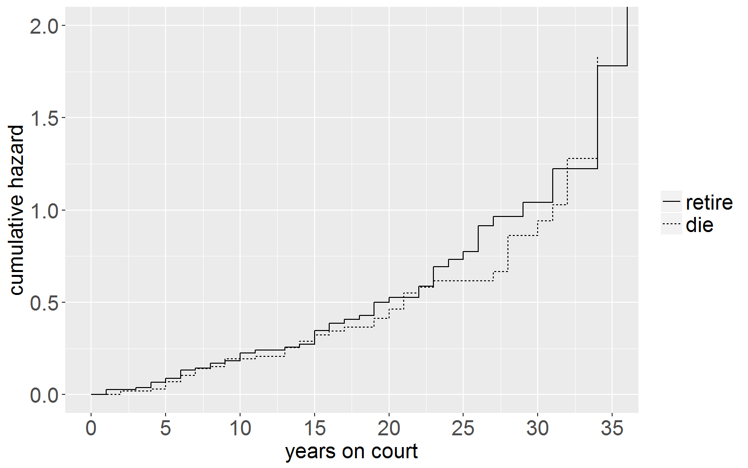
Kernel-Smoothed Hazard Function
We need a smoothing function for this graph. This one is taken from the R code for previous chapters.
smooth<- function(width, time, survive){
  n=length(time)
  lo=time[1] + width
  hi=time[n] - width
  npt=50
  inc=(hi-lo)/npt
  s=lo+t(c(1:npt))*inc
  slag = c(1, survive[1:n-1])
  h=1-survive/slag
  x1 = as.vector(rep(1, npt))%*%(t(time))
  x2 = t(s)%*%as.vector(rep(1,n))
  x = (x1 - x2) / width
  k=.75*(1-x*x)*(abs(x)<=1)
  lambda=(k%*%h)/width
  smoothed= list(x = s, y = lambda)
  return(smoothed)
}

# make the dataframe
df0 <- judgesLT[judgesLT$group == "retire",]
df1 <- judgesLT[judgesLT$group == "die",]
kSmooth0 <- smooth(6, df0$time, df0$surv) # need to play around with the width argument
kSmooth1 <- smooth(6, df1$time, df1$surv)
df_0 <- data.frame(x = drop(kSmooth0$x), y = drop(kSmooth0$y), group = "retire")[1:46,]
df_1 <- data.frame(x = drop(kSmooth1$x), y = drop(kSmooth1$y), group = "die")
kS <- rbind(df_0, df_1)

# plot it
 ggplot(kS, aes(x = x, y = y, group = group)) +
        geom_line(aes(linetype = group)) +
        xlab("Years on Court") + ylab("hazard") +
        coord_cartesian(xlim = c(0,30)) +
        scale_x_continuous(breaks = seq(0,30,5)) +
        theme(legend.text = element_text(size = 16),
              legend.title = element_blank(),
              axis.title.x = element_text(size = 16),
              axis.title.y = element_text(size = 16),
              axis.text.x = element_text(size = 16),
              axis.text.y = element_text(size = 16))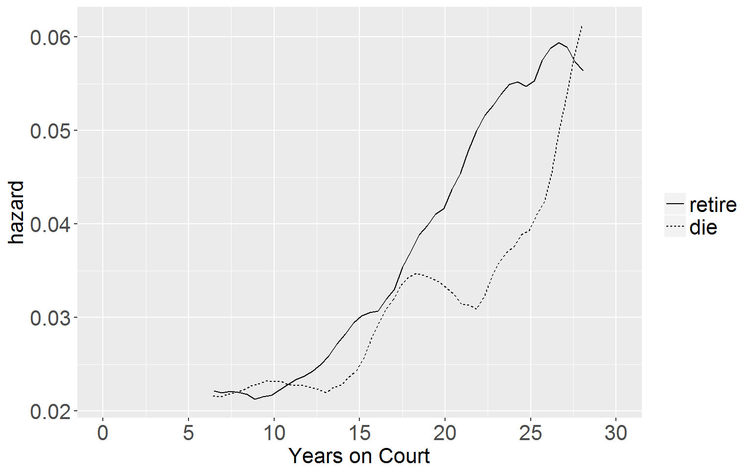
Table 15.7 p.592
Model A: Death Only
modA <- coxph(Surv(judges$tenure, judges$dead) ~ age + year, data = judges)
summary(modA)
## Call:
## coxph(formula = Surv(judges$tenure, judges$dead) ~ age + year,
## data = judges)
##
## n= 109, number of events= 47
##
## coef exp(coef) se(coef) z Pr(>|z|)
## age 0.067109 1.069412 0.023862 2.812 0.00492 **
## year -0.011602 0.988465 0.002894 -4.008 6.11e-05 ***
## ---
## Signif. codes: 0 '***' 0.001 '**' 0.01 '*' 0.05 '.' 0.1 ' ' 1
##
## exp(coef) exp(-coef) lower .95 upper .95
## age 1.0694 0.9351 1.0205 1.1206
## year 0.9885 1.0117 0.9829 0.9941
##
## Concordance= 0.675 (se = 0.051 )
## Rsquare= 0.165 (max possible= 0.96 )
## Likelihood ratio test= 19.61 on 2 df, p=5.529e-05
## Wald test = 18.58 on 2 df, p=9.249e-05
## Score (logrank) test = 19.05 on 2 df, p=7.291e-05Model B: Retire Only
modB <- coxph(Surv(judges$tenure, judges$retire) ~ age + year, data = judges)
summary(modB)
## Call:
## coxph(formula = Surv(judges$tenure, judges$retire) ~ age + year,
## data = judges)
##
## n= 109, number of events= 53
##
## coef exp(coef) se(coef) z Pr(>|z|)
## age 0.1061101 1.1119443 0.0257861 4.115 3.87e-05 ***
## year 0.0007141 1.0007144 0.0026432 0.270 0.787
## ---
## Signif. codes: 0 '***' 0.001 '**' 0.01 '*' 0.05 '.' 0.1 ' ' 1
##
## exp(coef) exp(-coef) lower .95 upper .95
## age 1.112 0.8993 1.0571 1.170
## year 1.001 0.9993 0.9955 1.006
##
## Concordance= 0.621 (se = 0.048 )
## Rsquare= 0.182 (max possible= 0.973 )
## Likelihood ratio test= 21.91 on 2 df, p=1.747e-05
## Wald test = 18.83 on 2 df, p=8.15e-05
## Score (logrank) test = 18.86 on 2 df, p=8.009e-05Model C: Death or Retire
modC <- coxph(Surv(judges$tenure, judges$leave) ~ age + year, data = judges)
summary(modC)
## Call:
## coxph(formula = Surv(judges$tenure, judges$leave) ~ age + year,
## data = judges)
##
## n= 109, number of events= 100
##
## coef exp(coef) se(coef) z Pr(>|z|)
## age 0.08606 1.08987 0.01766 4.874 1.09e-06 ***
## year -0.00522 0.99479 0.00188 -2.777 0.00549 **
## ---
## Signif. codes: 0 '***' 0.001 '**' 0.01 '*' 0.05 '.' 0.1 ' ' 1
##
## exp(coef) exp(-coef) lower .95 upper .95
## age 1.0899 0.9175 1.0528 1.1283
## year 0.9948 1.0052 0.9911 0.9985
##
## Concordance= 0.639 (se = 0.036 )
## Rsquare= 0.226 (max possible= 0.999 )
## Likelihood ratio test= 27.86 on 2 df, p=8.938e-07
## Wald test = 25.65 on 2 df, p=2.697e-06
## Score (logrank) test = 26.39 on 2 df, p=1.864e-06Compute hazard ratios for death-only and retirement-only models.
Hazard ratio, with age, for exiting the risk set by dying.
hazRatioAge_Death <- exp(coef(modA)[1])
hazRatioAge_Death
## age
## 1.069412Hazard ratio, with age, for exiting the risk set by retiring.
hazRatioAge_Retire <- exp(coef(modB)[1])
hazRatioAge_Retire
## age
## 1.11194410-year hazard ratios (as percent)
For death.
100*(hazRatioAge_Death^10-1)## age
## 95.63721For retirement.
100*(hazRatioAge_Retire^10-1)## age
## 188.9551Risk of dying on the job now compared to 100 years ago.
hazRatioYear_Death <- exp(coef(modA)[2])
hazRatioYear_Death
## year
## 0.9884654100*(hazRatioYear_Death^100-1)## year
## -68.65644Testing competing risks hypotheses
globalLogLik <- -2*logLik(modC)
sumEventSpecific <- -2*logLik(modA) + -2*logLik(modB)
diff <- globalLogLik - sumEventSpecific
diff
## 'log Lik.' 6.821101 (df=2)In order to test whether this difference in log likelihoods is significant we need to calculate the degrees of freedom for the relevant \(\chi^2\) distribution. There are two predictors in the model (p) and two competing event types, death and retirement (k). Therefore the degrees of freedom required is 2(2-1) = 2 x 1 = 2. We choose the critical value we want (here p < .05) and plug it into the \(\chi^2\) distribution on two degrees of freedom.
Critical value for p < .05
qchisq(.95,2) # for p < .05## [1] 5.991465qchisq(.99,2) # for p< .01## [1] 9.21034Because the difference in -2LL statistics (6.821) exceeds the p < .05 critical value of 5.99 we reject the null hypothesis that each predictor has identical coefficients across the events of death and retirement. In short: death and retirement are not equivalent ways of leaving office.
Wald Tests
betaAge_death <- coef(modA)[1]
betaAge_retire <- coef(modB)[1]
To get standard error we need to get a model summary.
sumDeath <- summary(modDeath <- coxph(Surv(judges$tenure, judges$dead) ~ age + year, data = judges))
seAge_death <- sumDeath$coefficients[1,3] # standard error year for death model

sumRetire <- summary(modRetire <- coxph(Surv(judges$tenure, judges$retire) ~ age + year, data = judges))
seAge_retire <- sumRetire$coefficients[1,3] # standard error year for retirement model
Now for the general Wald statistic
genWaldStat_Age <- (betaAge_death - betaAge_retire)^2 / (seAge_death^2 + seAge_retire^2)
genWaldStat_Age
## age
## 1.232326This does not exceed the p < .05 critical value
qchisq(.95,1)## [1] 3.841459… thus we cannot reject the null hypothesis of the effect of age on hazard of leaving differing across age and retirement event-types.
If we conduct the same procedure looking at differences, across event-types, in the effect of YEAR on hazard…
betaYear_death <- coef(modA)[2]
betaYear_retire <- coef(modB)[2]
seYear_death <- sumDeath$coefficients[2,3]
seYear_retire <- sumRetire$coefficients[2,3]
genWaldStat_Year <- (betaYear_death - betaYear_retire)^2 / (seYear_death^2 + seYear_retire^2)
genWaldStat_Year
## year
## 9.872623The test statistic exceeds the p < .01 critical value of
qchisq(.99,1)## [1] 6.634897……6.63 for a chi^2 distribution on one degree of freedom. Therefore we reject the null, concluding that the effect of YEAR differs across the two events. Combined with the non-significance of the coefficient for YEAR in the retirement model, we conclude that judges of any era were equally likely to step down, but that the risk of dying in office has declined.
Table 15.8 p.601
Model A
Read in the doctors dataset, create the vent variable, and split the single-entry dataset into a count-process dataset.
doctors <- read.csv("https://stats.idre.ucla.edu/stat/examples/alda/doctors.csv")
doctors$event <- 1 - doctors$censor
cutPoints <- sort(unique(doctors$exit[doctors$event == 1]))
longDocs <- survSplit(Surv(entry, exit, event)~.,
                      data = doctors,
                      cut = cutPoints,
                      end = "exit")
Now fit the model
modA <- coxph(Surv(entry, exit, event) ~ parttime + age + age:exit, data = longDocs)
summary(modA)
## Call:
## coxph(formula = Surv(entry, exit, event) ~ parttime + age + age:exit,
## data = longDocs)
##
## n= 57022, number of events= 396
##
## coef exp(coef) se(coef) z Pr(>|z|)
## parttime -1.347306 0.259940 0.276378 -4.875 1.09e-06 ***
## age 0.047811 1.048973 0.024211 1.975 0.04829 *
## age:exit -0.028666 0.971741 0.009059 -3.164 0.00155 **
## ---
## Signif. codes: 0 '***' 0.001 '**' 0.01 '*' 0.05 '.' 0.1 ' ' 1
##
## exp(coef) exp(-coef) lower .95 upper .95
## parttime 0.2599 3.8470 0.1512 0.4468
## age 1.0490 0.9533 1.0004 1.0999
## age:exit 0.9717 1.0291 0.9546 0.9891
##
## Concordance= 0.599 (se = 0.017 )
## Rsquare= 0.001 (max possible= 0.072 )
## Likelihood ratio test= 49.82 on 3 df, p=8.725e-11
## Wald test = 35.7 on 3 df, p=8.686e-08
## Score (logrank) test = 39.39 on 3 df, p=1.434e-08Model B
Create dataset with only the doctors who were hired during the measurement window
doctors0 <- doctors[doctors$entry == 0,]Once again, because we have an interaction, we need to split the dataset using the survSplit() function
cutPoints <- sort(unique(doctors$exit[doctors$event == 1]))
longDocs0 <- survSplit(Surv(entry, exit, event)~.,
                       data = doctors0,
                       cut = cutPoints,
                       end = "exit")
Now fit the model
modB <- coxph(Surv(entry, exit, event) ~ parttime + age + age:exit, data = longDocs0)
summary(modB)
## Call:
## coxph(formula = Surv(entry, exit, event) ~ parttime + age + age:exit,
## data = longDocs0)
##
## n= 13386, number of events= 57
##
## coef exp(coef) se(coef) z Pr(>|z|)
## parttime -0.170542 0.843208 0.520800 -0.327 0.743
## age 0.039797 1.040600 0.045529 0.874 0.382
## age:exit -0.003874 0.996133 0.044582 -0.087 0.931
##
## exp(coef) exp(-coef) lower .95 upper .95
## parttime 0.8432 1.186 0.3038 2.340
## age 1.0406 0.961 0.9518 1.138
## age:exit 0.9961 1.004 0.9128 1.087
##
## Concordance= 0.58 (se = 0.042 )
## Rsquare= 0 (max possible= 0.041 )
## Likelihood ratio test= 2.37 on 3 df, p=0.4996
## Wald test = 2.73 on 3 df, p=0.4346
## Score (logrank) test = 2.73 on 3 df, p=0.4346Model C
This is The incorrect model, ignoring the presence of late entrants. We are going to create the dataset incorrectly
First read in the dataset and create the event variable
doctorsIncorrect <- read.csv("https://stats.idre.ucla.edu/stat/examples/alda/doctors.csv")
doctorsIncorrect$event <- 1 - doctorsIncorrect$censor
Now we set all entry times to zero, reflecting total duration of tenure in the late-entry doctors (rather than duration of tenure while the window was open)…
doctorsIncorrect$entry <- 0Once again, because we have an interaction we need to split the dataset using the survSplit function
cutPoints <- sort(unique(doctorsIncorrect$exit[doctorsIncorrect$event == 1]))
longDocsIncorrect <- survSplit(Surv(entry, exit, event)~.,
                               data = doctorsIncorrect,
                               cut = cutPoints,
                               end = "exit")
Now fit the model
modC <- coxph(Surv(entry, exit, event) ~ parttime + age + age:exit, data = longDocsIncorrect)
summary(modC)
## Call:
## coxph(formula = Surv(entry, exit, event) ~ parttime + age + age:exit,
## data = longDocsIncorrect)
##
## n= 100331, number of events= 396
##
## coef exp(coef) se(coef) z Pr(>|z|)
## parttime -1.339382 0.262007 0.276487 -4.844 1.27e-06 ***
## age 0.097683 1.102613 0.019183 5.092 3.54e-07 ***
## age:exit -0.037045 0.963633 0.007788 -4.757 1.97e-06 ***
## ---
## Signif. codes: 0 '***' 0.001 '**' 0.01 '*' 0.05 '.' 0.1 ' ' 1
##
## exp(coef) exp(-coef) lower .95 upper .95
## parttime 0.2620 3.8167 0.1524 0.4505
## age 1.1026 0.9069 1.0619 1.1449
## age:exit 0.9636 1.0377 0.9490 0.9785
##
## Concordance= 0.61 (se = 0.017 )
## Rsquare= 0.001 (max possible= 0.044 )
## Likelihood ratio test= 56.44 on 3 df, p=3.38e-12
## Wald test = 49.6 on 3 df, p=9.728e-11
## Score (logrank) test = 51.9 on 3 df, p=3.14e-11Table 15.9 p.604
Model A
First read in the dataset.
monkeys <- read.csv("https://stats.idre.ucla.edu/stat/examples/alda/monkeys.csv")Now fit the model
modA <- coxph(Surv(SESSIONS, 1 - CENSOR) ~ INITIAL_AGE + BODYWT + FEMALE, data = monkeys)
summary(modA)
## Call:
## coxph(formula = Surv(SESSIONS, 1 - CENSOR) ~ INITIAL_AGE + BODYWT +
## FEMALE, data = monkeys)
##
## n= 123, number of events= 122
##
## coef exp(coef) se(coef) z Pr(>|z|)
## INITIAL_AGE 0.10636 1.11222 0.03386 3.141 0.00168 **
## BODYWT 0.11632 1.12336 0.02804 4.149 3.34e-05 ***
## FEMALE 0.37196 1.45058 0.19024 1.955 0.05056 .
## ---
## Signif. codes: 0 '***' 0.001 '**' 0.01 '*' 0.05 '.' 0.1 ' ' 1
##
## exp(coef) exp(-coef) lower .95 upper .95
## INITIAL_AGE 1.112 0.8991 1.0408 1.189
## BODYWT 1.123 0.8902 1.0633 1.187
## FEMALE 1.451 0.6894 0.9991 2.106
##
## Concordance= 0.659 (se = 0.035 )
## Rsquare= 0.181 (max possible= 1 )
## Likelihood ratio test= 24.55 on 3 df, p=1.916e-05
## Wald test = 26.42 on 3 df, p=7.786e-06
## Score (logrank) test = 25.69 on 3 df, p=1.105e-05Model B
Fit the model.
modB <- coxph(Surv(END_AGE, 1 - CENSOR) ~ INITIAL_AGE + BODYWT + FEMALE, data = monkeys)
summary(modB)
## Call:
## coxph(formula = Surv(END_AGE, 1 - CENSOR) ~ INITIAL_AGE + BODYWT +
## FEMALE, data = monkeys)
##
## n= 123, number of events= 122
##
## coef exp(coef) se(coef) z Pr(>|z|)
## INITIAL_AGE -0.09394 0.91034 0.03015 -3.116 0.001833 **
## BODYWT 0.10208 1.10748 0.02770 3.686 0.000228 ***
## FEMALE 0.29073 1.33741 0.18876 1.540 0.123516
## ---
## Signif. codes: 0 '***' 0.001 '**' 0.01 '*' 0.05 '.' 0.1 ' ' 1
##
## exp(coef) exp(-coef) lower .95 upper .95
## INITIAL_AGE 0.9103 1.0985 0.8581 0.9657
## BODYWT 1.1075 0.9030 1.0490 1.1693
## FEMALE 1.3374 0.7477 0.9238 1.9362
##
## Concordance= 0.691 (se = 0.034 )
## Rsquare= 0.212 (max possible= 1 )
## Likelihood ratio test= 29.38 on 3 df, p=1.867e-06
## Wald test = 26.87 on 3 df, p=6.265e-06
## Score (logrank) test = 28.18 on 3 df, p=3.337e-06Model C
To run Model C we need initial age on both sides of the equation. However the coxph() function won’t let you have the same predictor on both sides of the tilde. So we need to duplicate and rename it.
monkeys$init <- monkeys$INITIAL_AGE Now we can fit the model.
modC <- coxph(Surv(init, END_AGE, 1 - CENSOR) ~ INITIAL_AGE + BODYWT + FEMALE, data = monkeys)
summary(modC)
## Call:
## coxph(formula = Surv(init, END_AGE, 1 - CENSOR) ~ INITIAL_AGE +
## BODYWT + FEMALE, data = monkeys)
##
## n= 123, number of events= 122
##
## coef exp(coef) se(coef) z Pr(>|z|)
## INITIAL_AGE -0.01891 0.98127 0.03493 -0.541 0.588263
## BODYWT 0.10255 1.10799 0.02771 3.701 0.000215 ***
## FEMALE 0.31176 1.36583 0.18785 1.660 0.096993 .
## ---
## Signif. codes: 0 '***' 0.001 '**' 0.01 '*' 0.05 '.' 0.1 ' ' 1
##
## exp(coef) exp(-coef) lower .95 upper .95
## INITIAL_AGE 0.9813 1.0191 0.9163 1.051
## BODYWT 1.1080 0.9025 1.0494 1.170
## FEMALE 1.3658 0.7322 0.9451 1.974
##
## Concordance= 0.632 (se = 0.034 )
## Rsquare= 0.135 (max possible= 0.999 )
## Likelihood ratio test= 17.83 on 3 df, p=0.0004762
## Wald test = 17.83 on 3 df, p=0.0004772
## Score (logrank) test = 18.29 on 3 df, p=0.0003828Code provided by Llewellyn Mills PhD. Email llewmills@gmail.com for any feedback/questions.