R Textbook Examples Applied Longitudinal Data Analysis: Modeling Change and Event Occurrence by Judith D. Singer and John B. Willett Chapter 2: Exploring Longitudinal Data on Change
The comma separated text files linked on the main page have capitalized variable names. On this page the variable names are all lower case. For the appropriate lower case versions use tolerance1.txt and tolerance1_pp.txt.
Fig. 2.1, p. 18.
Inputting and printing the tolerance “person-level” data
tolerance <- read.table("https://stats.idre.ucla.edu/wp-content/uploads/2016/02/tolerance1.txt", sep=",", header=T)

print(tolerance)

     id tol11 tol12 tol13 tol14 tol15 male exposure
 1    9  2.23  1.79  1.90  2.12  2.66    0     1.54
 2   45  1.12  1.45  1.45  1.45  1.99    1     1.16
 3  268  1.45  1.34  1.99  1.79  1.34    1     0.90
 4  314  1.22  1.22  1.55  1.12  1.12    0     0.81
 5  442  1.45  1.99  1.45  1.67  1.90    0     1.13
 6  514  1.34  1.67  2.23  2.12  2.44    1     0.90
 7  569  1.79  1.90  1.90  1.99  1.99    0     1.99
 8  624  1.12  1.12  1.22  1.12  1.22    1     0.98
 9  723  1.22  1.34  1.12  1.00  1.12    0     0.81
10  918  1.00  1.00  1.22  1.99  1.22    0     1.21
11  949  1.99  1.55  1.12  1.45  1.55    1     0.93
12  978  1.22  1.34  2.12  3.46  3.32    1     1.59
13 1105  1.34  1.90  1.99  1.90  2.12    1     1.38
14 1542  1.22  1.22  1.99  1.79  2.12    0     1.44
15 1552  1.00  1.12  2.23  1.55  1.55    0     1.04
16 1653  1.11  1.11  1.34  1.55  2.12    0     1.25
Inputting and printing the tolerance “person-level” data
tolerance.pp <- read.table("https://stats.idre.ucla.edu/wp-content/uploads/2016/02/tolerance1_pp.txt", sep=",", header=T)

attach(tolerance.pp)

print(tolerance.pp[c(1:9, 76:80), ])
     id age tolerance male exposure time
 1    9  11      2.23    0     1.54    0
 2    9  12      1.79    0     1.54    1
 3    9  13      1.90    0     1.54    2
 4    9  14      2.12    0     1.54    3
 5    9  15      2.66    0     1.54    4
 6   45  11      1.12    1     1.16    0
 7   45  12      1.45    1     1.16    1
 8   45  13      1.45    1     1.16    2
 9   45  14      1.45    1     1.16    3
76 1653  11      1.11    0     1.25    0
77 1653  12      1.11    0     1.25    1
78 1653  13      1.34    0     1.25    2
79 1653  14      1.55    0     1.25    3
80 1653  15      2.12    0     1.25    4
Table 2.1, p. 20. Bivariate correlation among tolerance scores assessed on five occassions.
cor(tolerance[ , 2:6])
           tol11     tol12      tol13     tol14     tol15
tol11 1.00000000 0.6572937 0.06194915 0.1407631 0.2635371
tol12 0.65729370 1.0000000 0.24755116 0.2056198 0.3922781
tol13 0.06194915 0.2475512 1.00000000 0.5871742 0.5692116
tol14 0.14076312 0.2056198 0.58717422 1.0000000 0.8254566
tol15 0.26353705 0.3922781 0.56921163 0.8254566 1.0000000
Fig. 2.2, p. 25. Empirical growth plots.
library(lattice) # load lattice library for xyplot function

xyplot(tolerance ~ age | id, data=tolerance.pp, as.table=T)
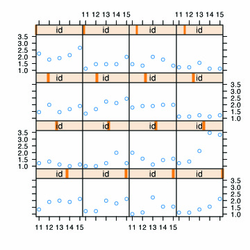
Fig. 2.3, p. 27. Smooth nonparametric trajectories superimposed on empirical growth plots.
xyplot(tolerance~age | id, data=tolerance.pp,
      prepanel = function(x, y) prepanel.loess(x, y, family="gaussian"),
      xlab = "Age", ylab = "Tolerance",
      panel = function(x, y) {
      panel.xyplot(x, y)
      panel.loess(x,y, family="gaussian") },
      ylim=c(0, 4), as.table=T)
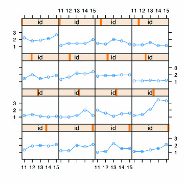
Table 2.2, p. 30. Fitting separate within person OLS regression models.
by(tolerance.pp, id, function(x) summary(lm(tolerance ~ time, data=x)))
tolerance.pp$id: 9

Call:
lm(formula = tolerance ~ time, data = x)

Residuals:
     1      2      3      4      5
 0.328 -0.231 -0.240 -0.139  0.282

Coefficients:
            Estimate Std. Error t value Pr(>|t|)
(Intercept)   1.9020     0.2519   7.549  0.00482 **
time          0.1190     0.1029   1.157  0.33105
---
Signif. codes:  0 `***' 0.001 `**' 0.01 `*' 0.05 `.' 0.1 ` ' 1

Residual standard error: 0.3253 on 3 degrees of freedom
Multiple R-Squared: 0.3085,     Adjusted R-squared: 0.07802
F-statistic: 1.339 on 1 and 3 DF,  p-value: 0.3311

------------------------------------------------------------------------------

<some output omitted>

------------------------------------------------------------------------------
tolerance.pp$id: 1653

Call:
lm(formula = tolerance ~ time, data = x)

Residuals:
    76     77     78     79     80
 0.156 -0.090 -0.106 -0.142  0.182

Coefficients:
            Estimate Std. Error t value Pr(>|t|)
(Intercept)  0.95400    0.13926   6.851  0.00637 **
time         0.24600    0.05685   4.327  0.02276 *
---
Signif. codes:  0 `***' 0.001 `**' 0.01 `*' 0.05 `.' 0.1 ` ' 1

Residual standard error: 0.1798 on 3 degrees of freedom
Multiple R-Squared: 0.8619,     Adjusted R-squared: 0.8159
F-statistic: 18.72 on 1 and 3 DF,  p-value: 0.02276
Fig. 2.4, p. 31.
# stem plot for the intercepts
int <- by(tolerance.pp, id, function(data)
                  coefficients(lm(tolerance ~ time, data = data))[[1]])
int <- unlist(int)
names(int) <- NULL
summary(int)

   Min. 1st Qu.  Median    Mean 3rd Qu.    Max.
  0.954   1.138   1.287   1.358   1.547   1.902

stem(int, scale=2)

Decimal point is 1 place to the left of the colon

    9 : 5
   10 : 03
   11 : 2489
   12 : 7
   13 : 1
   14 : 3
   15 : 448
   16 :
   17 : 3
   18 : 2
   19 : 0

# stem plot for fitted rate of change
rate <- by(tolerance.pp, id, function(data)
              coefficients(lm(tolerance ~ time, data = data))[[2]])
rate <- unlist(rate)
names(rate) <- NULL
summary(rate)

    Min.  1st Qu.   Median     Mean  3rd Qu.     Max.
-0.09800  0.02225  0.13100  0.13080  0.18980  0.63200

stem(rate, scale=2)

Decimal point is 1 place to the left of the colon

  -1 | 0
  -0 | 53
   0 | 2256
   1 | 24567
   2 | 457
   3 |
   4 |
   5 |
   6 | 3

# stem plot for R sq
rsq <- by(tolerance.pp, id, function(data)
             summary(lm(tolerance ~ time, data = data))$r.squared)
rsq <- unlist(rsq)
names(rsq) <- NULL
summary(rsq)

   Min. 1st Qu.  Median    Mean 3rd Qu.    Max.
0.01537 0.25050 0.39170 0.49100 0.79710 0.88640

stem(rsq, scale=2)

Decimal point is 1 place to the left of the colon

   0 : 27
   1 : 3
   2 : 55
   3 : 113
   4 : 5
   5 :
   6 : 8
   7 : 78
   8 : 6889
Fig. 2.5, p. 32. Fitted OLS trajectories superimposed on the empirical growth plots.
xyplot(tolerance ~ age | id, data=tolerance.pp,
  panel = function(x, y){
    panel.xyplot(x, y)
    panel.lmline(x, y)
  }, ylim=c(0, 4), as.table=T)
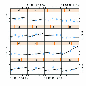
Fig. 2.6, p. 34. The collection of the trajectories of the raw data in the top panel; in the bottom panel is the collection of fitted OLS trajectories.
#plot of the raw data
interaction.plot(tolerance.pp$age, tolerance.pp$id, tolerance.pp$tolerance)
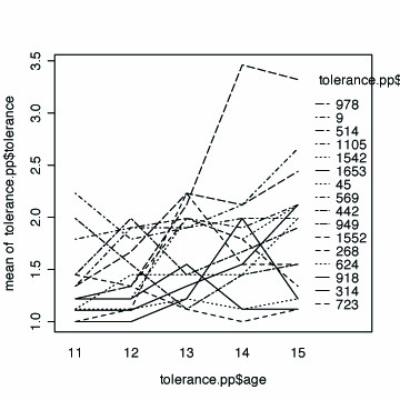
# fitting the linear model by id
fit <- by(tolerance.pp, id, function(bydata) fitted.values(lm(tolerance ~ time, data=bydata)))
fit <- unlist(fit)

# plotting the linear fit by id
interaction.plot(age, id, fit, xlab="age", ylab="tolerance")
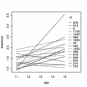
Table 2.3, p. 37 Descriptive statistics of the estimates obtained by fitting the linear model by id.
#obtaining the intercepts from linear model by id
ints <- by(tolerance.pp, tolerance.pp$id,
           function(data) coefficients(lm(tolerance ~ time, data=data))[[1]])
ints1 <- unlist(ints)
names(ints1) <- NULL
mean(ints1)
[1] 1.35775

sqrt(var(ints1))
[1] 0.2977792

#obtaining the slopes from linear model by id
slopes <- by(tolerance.pp, tolerance.pp$id,
             function(data) coefficients(lm(tolerance ~ time, data=data))[[2]])
slopes1 <- unlist(slopes)
names(slopes1) <- NULL
mean(slopes1)
[1] 0.1308125

sqrt(var(slopes1))
[1] 0.172296

cor( ints1, slopes1)
[1] -0.4481135
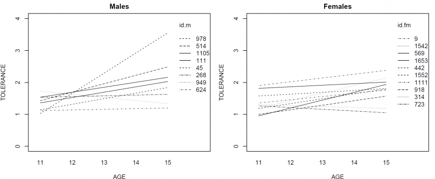
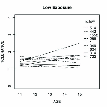
Fig. 2.7, 38 OLS fitted trajectories separated by levels of selected predictors. The two first panels are separated by gender; the two last are separated by levels of exposure.
# fitting the linear model by id, males only
tolm <- tolerance.pp[male == 1 , ]
fitmlist <- by(tolm, tolm$id, function(bydata) fitted.values(lm(tolerance ~ time, data=bydata)))
fitm <- unlist(fitmlist)

#appending the average for the whole group
lm.m <- fitted( lm(tolerance ~ time, data=tolm) )
names(lm.m) <- NULL
fit.m2 <- c(fitm, lm.m[1:5])
age.m <- c(tolm$age, seq(11,15))
id.m <- c(tolm$id, rep(111, 5))

#plotting the linear fit by id, males
#id.m=111 denotes the average value for males
interaction.plot(age.m, id.m, fit.m2, ylim=c(0, 4), xlab="AGE", ylab="TOLERANCE", lwd=1)
title(main="Males")
#fitting the linear model by id, females only
tol.pp.fm <- tolerance.pp[tolerance.pp$male == 0, ]
fit.fm <- by(tol.pp.fm, tol.pp.fm$id,
          function(data) fitted.values(lm(tolerance ~ time, data=data)))
fit.fm1 <- unlist(fit.fm)
names(fit.fm1) <- NULL

#appending the average for the whole group
lm.fm <- fitted( lm(tolerance ~ time, data=tol.pp.fm) )
names(lm.fm) <- NULL
fit.fm2 <- c(fit.fm1, lm.fm[1:5])
age.fm <- c(tol.pp.fm$age, seq(11,15))
id.fm <- c(tol.pp.fm$id, rep(1111, 5))

#plotting the linear fit by id, females
#id.fm=1111 denotes the average for females
interaction.plot(age.fm, id.fm, fit.fm2, ylim=c(0, 4), xlab="AGE", ylab="TOLERANCE", lwd=1)
title(main="Females")


#We can include both plot in the same graph
windows.options(width = 12, height = 5)
par(mfrow = c(1, 2), mar = c(4, 4, 2, 1))
interaction.plot(age.m, id.m, fit.m2, ylim=c(0, 4), xlab="AGE", ylab="TOLERANCE", lwd=1)
title(main="Males")
interaction.plot(age.fm, id.fm, fit.fm2, ylim=c(0, 4), xlab="AGE", ylab="TOLERANCE", lwd=1)
title(main="Females")


windows.options(reset = TRUE)
#fitting the linear model by id, low exposure
tol.pp.low <- tolerance.pp[tolerance.pp$exposure < 1.145 , ]
fit.low <- by(tol.pp.low, tol.pp.low$id,
          function(data) fitted.values(lm(tolerance ~ time, data=data)))
fit.low1 <- unlist(fit.low)
names(fit.low1) <- NULL

#appending the average for the whole group
lm.low <- fitted( lm(tolerance ~ time, data=tol.pp.low) )
names(lm.low) <- NULL
fit.low2 <- c(fit.low1, lm.low[1:5])
age.low <- c(tol.pp.low$age, seq(11,15))
id.low <- c(tol.pp.low$id, rep(1, 5))

#plotting the linear fit by id, low Exposure
#id.low=1 denotes the average for group
interaction.plot(age.low, id.low, fit.low2, ylim=c(0, 4), xlab="AGE", ylab="TOLERANCE", lwd=1)
title(main="Low Exposure")
#fitting the linear model by id, high exposure
tol.pp.hi <- tolerance.pp[tolerance.pp$exposure >= 1.145 , ]
fit.hi <- by(tol.pp.hi, tol.pp.hi$id,
          function(data) fitted.values(lm(tolerance ~ time, data=data)))
fit.hi1 <- unlist(fit.hi)
names(fit.hi1) <- NULL

#appending the average for the whole group
lm.hi <- fitted( lm(tolerance ~ time, data=tol.pp.hi) )
names(lm.hi) <- NULL
fit.hi2 <- c(fit.hi1, lm.hi[1:5])
age.hi <- c(tol.pp.hi$age, seq(11,15))
id.hi <- c(tol.pp.hi$id, rep(1, 5))

#plotting the linear fit by id, High Exposure
#id.hi=1 denotes the average for group
interaction.plot(age.hi, id.hi, fit.hi2, ylim=c(0, 4), xlab="AGE", ylab="TOLERANCE", lwd=1)
title(main="High Exposure")
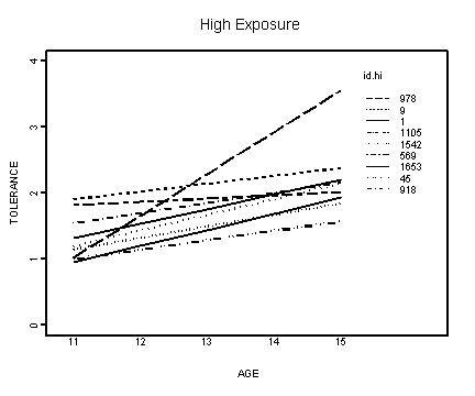
Fig. 2.8, p. 40. OLS estimates plotted against the predictors male and exposure.
#Using the slopes and intercepts from the linear model fitted by id
#generated for use in table 2.3
plot(tolerance$male, ints1, xlab="Male", ylab="Fitted initial status",
     xlim=c(0, 1), ylim=c(0.5, 2.5))
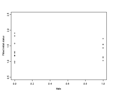
cor(tolerance$male, ints1)
[1] 0.008630119

plot(tolerance$exposure, ints1, xlab="Exposure", ylab="Fitted initial status",
     xlim=c(0, 2.5), ylim=c(0.5, 2.5))
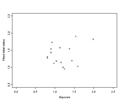
cor(tolerance$exposure, ints1)
[1] 0.2324426

plot(tolerance$male, slopes1, xlab="Male", ylab="Fitted rate of change",
     xlim=c(0, 1), ylim=c(-0.4, .8))
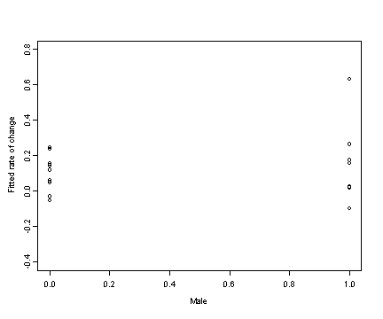
cor(tolerance$male, slopes1)
[1] 0.1935703

plot(tolerance$exposure, slopes1, xlab = "Exposure", ylab =
	"Fitted rate of change", xlim = c(0, 2.5), ylim = c(-0.2, 0.8))
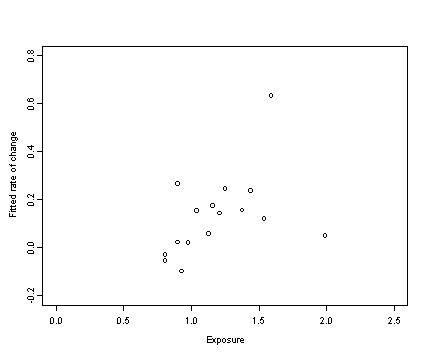
cor(tolerance$exposure, slopes1)
[1] 0.4420925