R Textbook Examples Applied Longitudinal Data Analysis: Modeling Change and Event Occurrence by Judith D. Singer and John B. Willett Chapter 4: Doing Data Analysis with the Multilevel Model for Change
#Read data and attach dataset
alcohol1 <- read.table("https://stats.idre.ucla.edu/stat/r/examples/alda/data/alcohol1_pp.txt", header=T, sep=",")
attach(alcohol1)
Fig. 4.1, p. 77. Empirical growth plots with superimposed OLS trajectories.
library(lattice)

xyplot(alcuse~age | id,
   data=alcohol1[alcohol1$id %in% c(4, 14, 23, 32, 41, 56, 65, 82), ],
   panel=function(x,y){
	panel.xyplot(x, y)
	panel.lmline(x,y)
}, ylim=c(-1, 4), as.table=T)
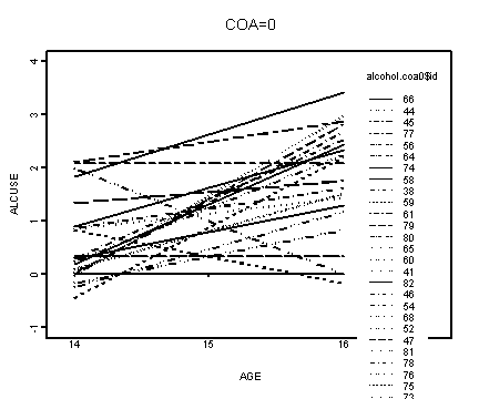
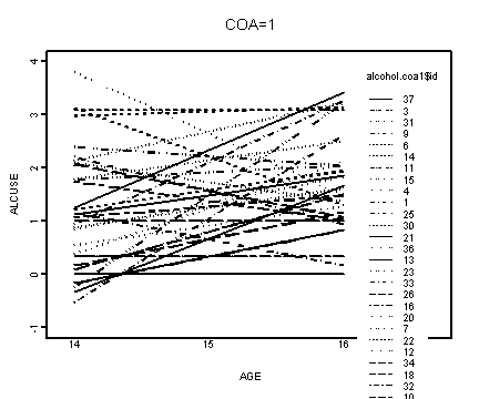
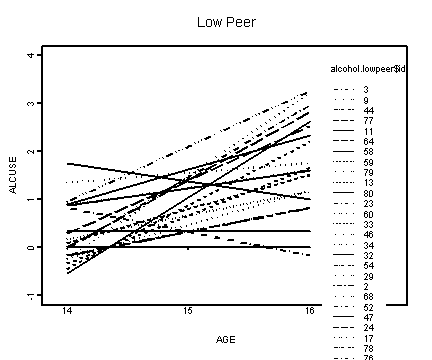
Fig. 4.2, p.79. Fitted OLS trajectories displayed separately by coa status and peer levels.
Upper left panel, coa=0.
alcohol.coa0 <- alcohol1[alcohol1$coa==0, ]

#fitting the linear model by id
f.coa0 <- by(alcohol.coa0, alcohol.coa0$id,
                function(data) fitted(lm(alcuse~age, data=data)))
#transforming f.coa from a list to a vector and
#stripping of the names of the elements in the vector
f.coa0 <- unlist(f.coa0)
names(f.coa0) <- NULL

#plotting the linear fit by id
interaction.plot(alcohol.coa0$age, alcohol.coa0$id, f.coa0,
                 xlab="AGE", ylab="ALCUSE", ylim=c(-1, 4), lwd=1)
title("COA=0")
Upper right panel, coa=1.
alcohol.coa1 <- alcohol1[alcohol1$coa==1, ]

#fitting the linear model by id
f.coa1 <- by(alcohol.coa1, alcohol.coa1$id,
             function(data) fitted(lm(alcuse~age, data=data)))
#transforming f.coa1 from a list to a vector and
#stripping of the names of the elements in the vector
f.coa1 <- unlist(f.coa1)
names(f.coa1) <- NULL

#plotting the linear fit by id
interaction.plot(alcohol.coa1$age, alcohol.coa1$id, f.coa1,
                 xlab="AGE", ylab="ALCUSE", ylim=c(-1, 4), lwd=1)
title("COA=1")
Obtaining the mean of peer and graphing the lower left panel, peer<=1.01756.
mean(alcohol1$peer)
[1] 1.01756

alcohol.lowpeer <- alcohol1[alcohol1$peer<=1.01756, ]

#fitting the linear model by id
f.lowpeer <- by(alcohol.lowpeer, alcohol.lowpeer$id,
             function(data) fitted(lm(alcuse~age, data=data)))
#transforming f.lowpeer from a list to a vector and
#stripping of the names of the elements in the vector
f.lowpeer <- unlist(f.lowpeer)
names(f.lowpeer) <- NULL

#plotting the linear fit by id
interaction.plot(alcohol.lowpeer$age, alcohol.lowpeer$id, f.lowpeer,
                 xlab="AGE", ylab="ALCUSE", ylim=c(-1, 4), lwd=1)
title("Low Peer")
Lower right panel, peer>1.01756.
alcohol.hipeer <- alcohol1[alcohol1$peer>1.01756, ]

#fitting the linear model by id
f.hipeer <- by(alcohol.hipeer, alcohol.hipeer$id,
               function(data) fitted(lm(alcuse~age, data=data)))
#transforming f.hipeer from a list to a vector and
#stripping of the names of the elements in the vector
f.hipeer <- unlist(f.hipeer)
names(f.hipeer) <- NULL

#plotting the linear fit by id
interaction.plot(alcohol.hipeer$age, alcohol.hipeer$id, f.hipeer,
                 xlab="AGE", ylab="ALCUSE", ylim=c(-1, 4), lwd=1)
title("High Peer")
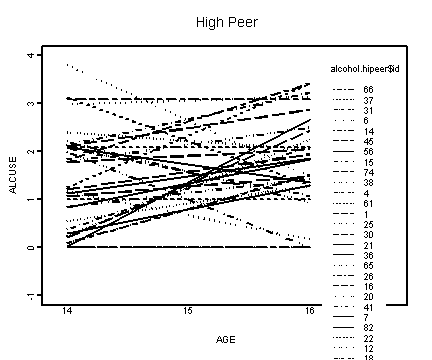
Table 4.1, p. 94-95.
#Model A
library(nlme)

model.a <- lme(alcuse~ 1, alcohol1, random= ~1 |id)
summary(model.a)

Linear mixed-effects model fit by REML
 Data: alcohol1
       AIC      BIC    logLik
  679.0049 689.5087 -336.5025

Random effects:
 Formula: ~1 | id
        (Intercept)  Residual
StdDev:   0.7570578 0.7494974

Fixed effects: alcuse ~ 1
                Value  Std.Error  DF  t-value p-value
(Intercept) 0.9219549 0.09629638 164 9.574139       0

Standardized Within-Group Residuals:
       Min         Q1        Med         Q3        Max
-1.8892070 -0.3079143 -0.3029178  0.6110925  2.8562135

Number of Observations: 246
Number of Groups: 82

#Model B
model.b <- lme(alcuse ~ age_14 , data=alcohol1, random= ~ age_14 | id, method="ML")
summary(model.b)

Linear mixed-effects model fit by maximum likelihood
 Data: alcohol1
       AIC     BIC    logLik
  648.6111 669.643 -318.3055

Random effects:
 Formula: ~age_14 | id
 Structure: General positive-definite, Log-Cholesky parametrization
            StdDev    Corr
(Intercept) 0.7901617 (Intr)
age_14      0.3888470 -0.223
Residual    0.5807690

Fixed effects: alcuse ~ age_14
                Value  Std.Error  DF  t-value p-value
(Intercept) 0.6513035 0.10551005 163 6.172905       0
age_14      0.2706514 0.06271014 163 4.315912       0
 Correlation:
       (Intr)
age_14 -0.441

Standardized Within-Group Residuals:
        Min          Q1         Med          Q3         Max
-2.47998885 -0.38401088 -0.07553389  0.39001356  2.50684931

Number of Observations: 246
Number of Groups: 82
#Model C
model.c <- lme(alcuse ~ coa*age_14 , data=alcohol1, random= ~ age_14 | id, method="ML")
summary(model.c)

Linear mixed-effects model fit by maximum likelihood
 Data: alcohol1
       AIC      BIC    logLik
  637.2026 665.2453 -310.6013

Random effects:
 Formula: ~age_14 | id
 Structure: General positive-definite, Log-Cholesky parametrization
            StdDev    Corr
(Intercept) 0.6982690 (Intr)
age_14      0.3880684 -0.219
Residual    0.5807688

Fixed effects: alcuse ~ coa * age_14
                 Value  Std.Error  DF   t-value p-value
(Intercept)  0.3159517 0.13177099 162  2.397734  0.0176
coa          0.7432120 0.19616697  80  3.788671  0.0003
age_14       0.2929552 0.08492089 162  3.449742  0.0007
coa:age_14  -0.0494299 0.12642140 162 -0.390993  0.6963
 Correlation:
           (Intr) coa    age_14
coa        -0.672
age_14     -0.460  0.309
coa:age_14  0.309 -0.460 -0.672

Standardized Within-Group Residuals:
       Min         Q1        Med         Q3        Max
-2.5480533 -0.3879877 -0.1057547  0.3602391  2.3960739

Number of Observations: 246
Number of Groups: 82
#Model D
model.d <- lme(alcuse ~ coa*age_14+peer*age_14 , data=alcohol1, random= ~ age_14 | id, method="ML")
summary(model.d)

Linear mixed-effects model fit by maximum likelihood
 Data: alcohol1
       AIC     BIC    logLik
  608.6906 643.744 -294.3453

Random effects:
 Formula: ~age_14 | id
 Structure: General positive-definite, Log-Cholesky parametrization
            StdDev    Corr
(Intercept) 0.4908199 (Intr)
age_14      0.3729821 -0.033
Residual    0.5807668

Fixed effects: alcuse ~ coa * age_14 + peer * age_14
                 Value  Std.Error  DF   t-value p-value
(Intercept) -0.3165142 0.14990058 161 -2.111494  0.0363
coa          0.5791651 0.16450407  79  3.520673  0.0007
age_14       0.4294286 0.11510211 161  3.730849  0.0003
peer         0.6942956 0.11291811  79  6.148665  0.0000
coa:age_14  -0.0140319 0.12631549 161 -0.111086  0.9117
age_14:peer -0.1498150 0.08670489 161 -1.727873  0.0859
 Correlation:
            (Intr) coa    age_14 peer   c:g_14
coa         -0.371
age_14      -0.436  0.162
peer        -0.686 -0.162  0.299
coa:age_14   0.162 -0.436 -0.371  0.071
age_14:peer  0.299  0.071 -0.686 -0.436 -0.162

Standardized Within-Group Residuals:
        Min          Q1         Med          Q3         Max
-2.59555028 -0.40005029 -0.07769136  0.46002837  2.29373867

Number of Observations: 246
Number of Groups: 82
#Model E
model.e <- lme(alcuse ~ coa+peer*age_14 , data=alcohol1, random= ~ age_14 | id, method="ML")
summary(model.e)

Linear mixed-effects model fit by maximum likelihood
 Data: alcohol1
       AIC      BIC    logLik
  606.7033 638.2513 -294.3516

Random effects:
 Formula: ~age_14 | id
 Structure: General positive-definite, Log-Cholesky parametrization
            StdDev    Corr
(Intercept) 0.4908384 (Intr)
age_14      0.3730386 -0.034
Residual    0.5807689

Fixed effects: alcuse ~ coa + peer * age_14
                 Value  Std.Error  DF   t-value p-value
(Intercept) -0.3138215 0.14762315 162 -2.125828  0.0350
coa          0.5711970 0.14773604  79  3.866335  0.0002
peer         0.6951827 0.11240363  79  6.184699  0.0000
age_14       0.4246867 0.10667952 162  3.980958  0.0001
peer:age_14 -0.1513771 0.08538528 162 -1.772872  0.0781
 Correlation:
            (Intr) coa    peer   age_14
coa         -0.338
peer        -0.709 -0.146
age_14      -0.410  0.000  0.351
peer:age_14  0.334  0.000 -0.431 -0.814

Standardized Within-Group Residuals:
       Min         Q1        Med         Q3        Max
-2.5955443 -0.4041410 -0.0835195  0.4554950  2.2997515

Number of Observations: 246
Number of Groups: 82
#Model F
model.f <- lme(alcuse ~ coa+cpeer*age_14 , data=alcohol1, random= ~ age_14 | id, method="ML")
summary(model.f)

Linear mixed-effects model fit by maximum likelihood
 Data: alcohol1
       AIC      BIC    logLik
  606.7033 638.2513 -294.3516

Random effects:
 Formula: ~age_14 | id
 Structure: General positive-definite, Log-Cholesky parametrization
            StdDev    Corr
(Intercept) 0.4908389 (Intr)
age_14      0.3730381 -0.034
Residual    0.5807690

Fixed effects: alcuse ~ coa + cpeer * age_14
                  Value  Std.Error  DF   t-value p-value
(Intercept)   0.3938745 0.10460706 162  3.765276  0.0002
coa           0.5711970 0.14773612  79  3.866333  0.0002
cpeer         0.6951827 0.11240368  79  6.184696  0.0000
age_14        0.2705847 0.06189978 162  4.371336  0.0000
cpeer:age_14 -0.1513771 0.08538523 162 -1.772873  0.0781
 Correlation:
             (Intr) coa    cpeer  age_14
coa          -0.637
cpeer         0.094 -0.146
age_14       -0.336  0.000  0.000
cpeer:age_14  0.000  0.000 -0.431  0.001

Standardized Within-Group Residuals:
        Min          Q1         Med          Q3         Max
-2.59554441 -0.40414064 -0.08351877  0.45549526  2.29975184

Number of Observations: 246
Number of Groups: 82
#Model G
model.g <- lme(alcuse ~ ccoa+cpeer*age_14 , data=alcohol1, random= ~ age_14 | id, method="ML")
summary(model.g)

Linear mixed-effects model fit by maximum likelihood
 Data: alcohol1
       AIC      BIC    logLik
  606.7033 638.2513 -294.3516

Random effects:
 Formula: ~age_14 | id
 Structure: General positive-definite, Log-Cholesky parametrization
            StdDev    Corr
(Intercept) 0.4908386 (Intr)
age_14      0.3730384 -0.034
Residual    0.5807690

Fixed effects: alcuse ~ ccoa + cpeer * age_14
                  Value  Std.Error  DF   t-value p-value
(Intercept)   0.6514843 0.08060971 162  8.081959  0.0000
ccoa          0.5711970 0.14773606  79  3.866334  0.0002
cpeer         0.6951827 0.11240365  79  6.184698  0.0000
age_14        0.2705847 0.06189981 162  4.371334  0.0000
cpeer:age_14 -0.1513771 0.08538526 162 -1.772872  0.0781
 Correlation:
             (Intr) ccoa   cpeer  age_14
ccoa          0.000
cpeer         0.001 -0.146
age_14       -0.436  0.000  0.000
cpeer:age_14  0.000  0.000 -0.431  0.001

Standardized Within-Group Residuals:
        Min          Q1         Med          Q3         Max
-2.59554430 -0.40414090 -0.08351925  0.45549506  2.29975158

Number of Observations: 246
Number of Groups: 82
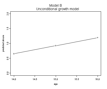
Fig. 4.3, p. 99. Model B
fixef.b <- fixef(model.b)
fit.b <- fixef.b[[1]] + alcohol1$age_14[1:3]*fixef.b[[2]]
plot(alcohol1$age[1:3], fit.b, ylim=c(0, 2), type="b",
     ylab="predicted alcuse", xlab="age")
title("Model B \n Unconditional growth model")
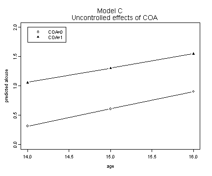
Model C.
fixef.c <- fixef(model.c)
fit.c0 <- fixef.c[[1]] + alcohol1$age_14[1:3]*fixef.c[[3]]
fit.c1 <- fixef.c[[1]] + fixef.c[[2]] +
          alcohol1$age_14[1:3]*fixef.c[[3]] +
          alcohol1$age_14[1:3]*fixef.c[[4]]
plot(alcohol1$age[1:3], fit.c0, ylim=c(0, 2), type="b",
     ylab="predicted alcuse", xlab="age")
lines(alcohol1$age[1:3], fit.c1, type="b", pch=17)
title("Model C \n Uncontrolled effects of COA")
legend(14, 2, c("COA=0", "COA=1"))
Model E.
fixef.e <- fixef(model.e)
fit.ec0p0 <- fixef.e[[1]] + .655*fixef.e[[3]] +
             alcohol1$age_14[1:3]*fixef.e[[4]] +
             .655*alcohol1$age_14[1:3]*fixef.e[[5]]
fit.ec0p1 <- fixef.e[[1]] + 1.381*fixef.e[[3]] +
             alcohol1$age_14[1:3]*fixef.e[[4]] +
             1.381*alcohol1$age_14[1:3]*fixef.e[[5]]
fit.ec1p0 <- fixef.e[[1]] + fixef.e[[2]] + .655*fixef.e[[3]] +
             alcohol1$age_14[1:3]*fixef.e[[4]] +
             .655*alcohol1$age_14[1:3]*fixef.e[[5]]
fit.ec1p1 <- fixef.e[[1]] + fixef.e[[2]] + 1.381*fixef.e[[3]] +
             alcohol1$age_14[1:3]*fixef.e[[4]] +
             1.381*alcohol1$age_14[1:3]*fixef.e[[5]]
plot(alcohol1$age[1:3], fit.ec0p0, ylim=c(0, 2), type="b",
     ylab="predicted alcuse", xlab="age", pch=2)
lines(alcohol1$age[1:3], fit.ec0p1, type="b", pch=0)
lines(alcohol1$age[1:3], fit.ec1p0, type="b", pch=17)
lines(alcohol1$age[1:3], fit.ec1p1, type="b", pch=15)
title("Model E \n *Final* model for the controlled effects of COA")
legend(14, 2, c("COA=0, low peer", "COA=0, high peer",
       "COA=1, low peer", "COA=1, high peer"))
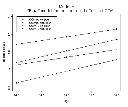
Fig. 4.4–skipped
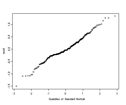
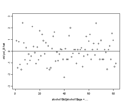
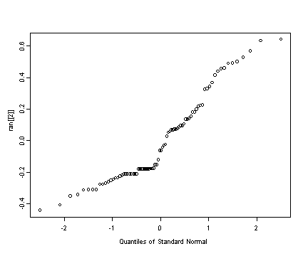
Fig. 4.5, p. 131. Normality assumption plots.
Upper left panel
#creating the residuals (epsilon.hat)
resid <- residuals(model.f)
qqnorm(resid)
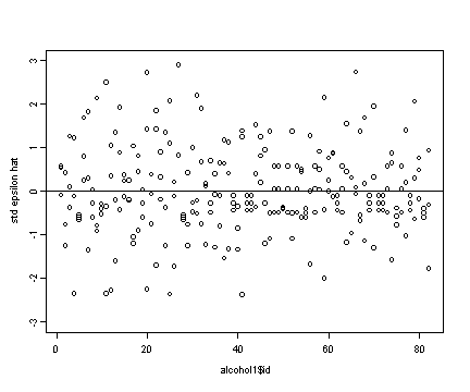
Upper right panel
#creating the standardized residual (std epsilon.hat)
resid.std <- resid/sd(resid)
plot(alcohol1$id, resid.std, ylim=c(-3, 3), ylab="std epsilon hat")
abline(h=0)
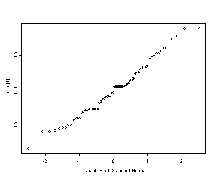
Middle left panel
#extracting the random effects of model f
ran <- random.effects(model.f)
qqnorm(ran[[1]])
Middle right panel
#standardizing the ksi0i.hat
ran1.std <- ran[[1]]/sd(ran[[1]])
plot(alcohol1$id[alcohol1$age==14], ran1.std, ylim=c(-3, 3), ylab="std psi_0i hat")
abline(h=0)
Lower left panel
qqnorm(ran[[2]])
Lower right panel
#standardizing the ksi1i.hat
ran2.std <- ran[[2]]/sd(ran[[2]])
plot(id[alcohol1$age==14], ran2.std, ylim=c(-3, 3), ylab="std psi_1i hat")
abline(h=0)
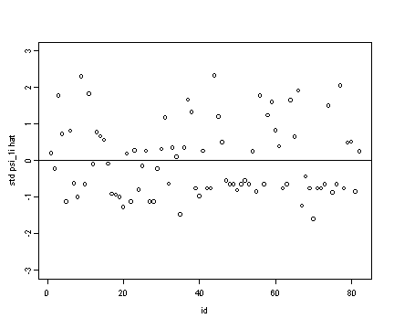
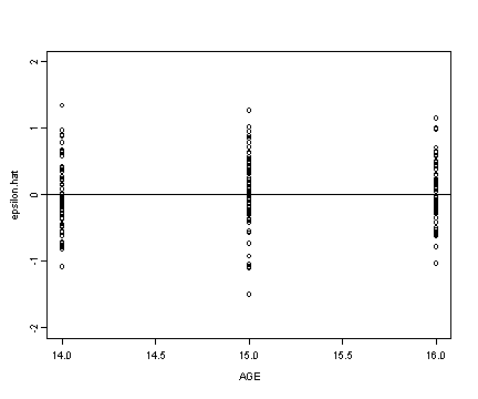
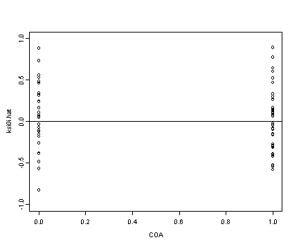
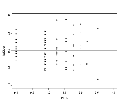
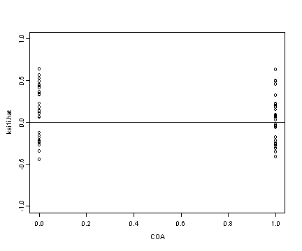
Fig. 4.6, p. 133. Homoscedasticity plots.
Upper panel
plot(alcohol1$age, resid, ylim=c(-2, 2), ylab="epsilon.hat",
     xlab="AGE")
abline(h=0)
Middle left panel
plot(alcohol1$coa[alcohol1$age==14], ran[[1]], ylim=c(-1, 1),
     ylab="ksi0i.hat", xlab="COA")
abline(h=0)
Middle right panel
plot(alcohol1$peer[alcohol1$age==14], ran[[1]], ylim=c(-1, 1),
     xlim=c(0, 3), ylab="ksi0i.hat", xlab="PEER")
abline(h=0)
Lower left panel
plot(alcohol1$coa[alcohol1$age==14], ran[[2]], ylim=c(-1, 1),
     ylab="ksi1i.hat", xlab="COA")
abline(h=0)
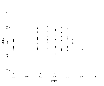
Lower right panel
plot(alcohol1$peer[alcohol1$age==14], ran[[2]], ylim=c(-1, 1),
     xlim=c(0, 3), ylab="ksi1i.hat", xlab="PEER")
abline(h=0)