Applied Longitudinal Data Analysis: Modeling Change and Event Occurrence by Judith D. Singer and John B. Willett Chapter 5: Treating TIME More Flexibly
Inputting the reading data set.
reading <- read.table("https://stats.idre.ucla.edu/stat/r/examples/alda/data/reading_pp.txt", header=T, sep=",")
Table 5.1, p. 141.
reading[reading$id %in% c(4, 27, 31, 33, 41, 49, 69, 77, 87), ]

    id wave agegrp       age piat agegrp.c      age.c
 10  4    1    6.5  6.000000   18        0 -0.5000000
 11  4    2    8.5  8.500000   31        2  2.0000000
 12  4    3   10.5 10.666667   50        4  4.1666667
 79 27    1    6.5  6.250000   19        0 -0.2500000
 80 27    2    8.5  9.166667   36        2  2.6666667
 81 27    3   10.5 10.916667   57        4  4.4166667
 91 31    1    6.5  6.333333   18        0 -0.1666667
 92 31    2    8.5  8.833333   31        2  2.3333333
 93 31    3   10.5 10.916667   51        4  4.4166667
 97 33    1    6.5  6.333333   18        0 -0.1666667
 98 33    2    8.5  8.916667   34        2  2.4166667
 99 33    3   10.5 10.750000   29        4  4.2500000
121 41    1    6.5  6.333333   18        0 -0.1666667
122 41    2    8.5  8.750000   28        2  2.2500000
123 41    3   10.5 10.833333   36        4  4.3333333
145 49    1    6.5  6.500000   19        0  0.0000000
146 49    2    8.5  8.750000   32        2  2.2500000
147 49    3   10.5 10.666667   48        4  4.1666667
205 69    1    6.5  6.666667   26        0  0.1666667
206 69    2    8.5  9.166667   47        2  2.6666667
207 69    3   10.5 11.333333   45        4  4.8333333
229 77    1    6.5  6.833333   17        0  0.3333333
230 77    2    8.5  8.083333   19        2  1.5833333
231 77    3   10.5 10.000000   28        4  3.5000000
259 87    1    6.5  6.916667   22        0  0.4166667
260 87    2    8.5  9.416667   49        2  2.9166667
261 87    3   10.5 11.500000   64        4  5.0000000
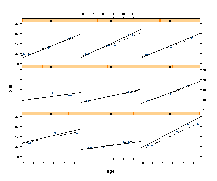
Fig. 5.1, p. 143. Empirical change plots with superimposed OLS trajectories. The +’s and solid lines correspond to time using the child’s target age at data collection, whereas the dots and dashed lines correspond to time using the child’s observed age.
library(lattice)

xyplot(piat~age | id,
   data=reading[reading$id %in% c(4, 27, 31, 33, 41, 49, 69, 77, 87), ],
    panel=function(x,y, subscripts){panel.xyplot(x, y, pch=16)
	panel.lmline(x,y, lty=4)
    panel.xyplot(reading$agegrp[subscripts], y, pch=3)
	panel.lmline(reading$agegrp[subscripts],y) },
    ylim=c(0, 80), as.table=T, subscripts=T)
Creating the centered variables called agegrp.c and age.c, p. 144.
mat2 <- reading[ ,3:4]-6.5
dimnames(mat2)[[2]] <- c("agegrp.c", "age.c")
reading <- cbind(reading, mat2)
Table 5.2, p. 145. Note: The degres of freedom used to in the calculations of the intercept is different from the results in the book and this difference in partitioning results also in slight differences in the standard error of the estimates.
#Using the agegrp variable.
library(nlme)

lme.agegrp <- lme(piat ~ agegrp.c, reading, random= ~ agegrp | id, method="ML")
summary(lme.agegrp)

Linear mixed-effects model fit by maximum likelihood
 Data: reading
       AIC      BIC    logLik
  1831.949 1853.473 -909.9746

Random effects:
 Formula: ~agegrp | id
 Structure: General positive-definite, Log-Cholesky parametrization
            StdDev    Corr
(Intercept) 13.244933 (Intr)
agegrp       2.096994 -0.97
Residual     5.200308

Fixed effects: piat ~ agegrp.c
                Value Std.Error  DF  t-value p-value
(Intercept) 21.162921 0.6165805 177 34.32304       0
agegrp.c     5.030899 0.2967329 177 16.95430       0
 Correlation:
         (Intr)
agegrp.c -0.316

Standardized Within-Group Residuals:
       Min         Q1        Med         Q3        Max
-2.6585175 -0.5418435 -0.1434177  0.3871955  3.3133003

Number of Observations: 267
Number of Groups: 89

#Using the age variable.
lme.age <- lme(piat ~ age.c, reading, random= ~ age | id, method="ML")
summary(lme.age)

Linear mixed-effects model fit by maximum likelihood
 Data: reading
       AIC      BIC    logLik
  1815.896 1837.419 -901.9478

Random effects:
 Formula: ~age | id
 Structure: General positive-definite, Log-Cholesky parametrization
            StdDev    Corr
(Intercept) 10.668937 (Intr)
age          1.816985 -0.985
Residual     5.238946

Fixed effects: piat ~ age.c
                Value Std.Error  DF  t-value p-value
(Intercept) 21.060816 0.5614177 177 37.51363       0
age.c        4.540021 0.2616162 177 17.35375       0
 Correlation:
      (Intr)
age.c -0.287

Standardized Within-Group Residuals:
       Min         Q1        Med         Q3        Max
-3.0068407 -0.4948682 -0.1369712  0.4095972  3.7274111

Number of Observations: 267
Number of Groups: 89
Inputting the wages data set.
wages <- read.table("https://stats.idre.ucla.edu/stat/r/examples/alda/data/wages_pp.txt", header=T, sep=",")
Table 5.3, p. 147.
wages[wages$id %in% c(206, 332, 1028), c(1, 3, 2, 6, 8, 10)]

      id exper   lnw black hgc uerate
 75  206 1.874 2.028     0  10  9.200
 76  206 2.814 2.297     0  10 11.000
 77  206 4.314 2.482     0  10  6.295
197  332 0.125 1.630     0   8  7.100
198  332 1.625 1.476     0   8  9.600
199  332 2.413 1.804     0   8  7.200
200  332 3.393 1.439     0   8  6.195
201  332 4.470 1.748     0   8  5.595
202  332 5.178 1.526     0   8  4.595
203  332 6.082 2.044     0   8  4.295
204  332 7.043 2.179     0   8  3.395
205  332 8.197 2.186     0   8  4.395
206  332 9.092 4.035     0   8  6.695
466 1028 0.004 0.872     1   8  9.300
467 1028 0.035 0.903     1   8  7.400
468 1028 0.515 1.389     1   8  7.300
469 1028 1.483 2.324     1   8  7.400
470 1028 2.141 1.484     1   8  6.295
471 1028 3.161 1.705     1   8  5.895
472 1028 4.103 2.343     1   8  6.900
Table 5.4, p. 149.
#Model A
model.a <- lme(lnw~exper, wages, random= ~exper | id, method="ML")
summary(model.a)

Linear mixed-effects model fit by maximum likelihood
 Data: wages
       AIC     BIC    logLik
  4933.394 4973.98 -2460.697

Random effects:
 Formula: ~exper | id
 Structure: General positive-definite, Log-Cholesky parametrization
            StdDev     Corr
(Intercept) 0.23295542 (Intr)
exper       0.04154474 -0.301
Residual    0.30839044

Fixed effects: lnw ~ exper
                Value   Std.Error   DF   t-value p-value
(Intercept) 1.7156039 0.010798215 5513 158.87848       0
exper       0.0456807 0.002341936 5513  19.50555       0
 Correlation:
      (Intr)
exper -0.565

Standardized Within-Group Residuals:
        Min          Q1         Med          Q3         Max
-4.20113322 -0.52073077 -0.03159151  0.44063202  7.03696490

Number of Observations: 6402
Number of Groups: 888

#Model B
model.b <- update(model.a, lnw~exper*hgc.9+exper*black)
summary(model.b)

Linear mixed-effects model fit by maximum likelihood
 Data: wages
       AIC      BIC    logLik
  4893.751 4961.395 -2436.876

Random effects:
 Formula: ~exper | id
 Structure: General positive-definite, Log-Cholesky parametrization
            StdDev     Corr
(Intercept) 0.22748211 (Intr)
exper       0.04044512 -0.31
Residual    0.30853484

Fixed effects: lnw ~ exper + hgc.9 + black + exper:hgc.9 + exper:black
                 Value   Std.Error   DF   t-value p-value
(Intercept)  1.7171385 0.012548264 5511 136.84271  0.0000
exper        0.0493428 0.002632917 5511  18.74074  0.0000
hgc.9        0.0349201 0.007885174  885   4.42858  0.0000
black        0.0153954 0.023937728  885   0.64315  0.5203
exper:hgc.9  0.0012794 0.001723983 5511   0.74213  0.4580
exper:black -0.0182129 0.005501727 5511  -3.31040  0.0009
 Correlation:
            (Intr) exper  hgc.9  black  exp:.9
exper       -0.575
hgc.9        0.071 -0.020
black       -0.523  0.301 -0.020
exper:hgc.9 -0.019 -0.003 -0.578  0.011
exper:black  0.275 -0.478  0.011 -0.573 -0.023

Standardized Within-Group Residuals:
        Min          Q1         Med          Q3         Max
-4.26907899 -0.51809173 -0.03347663  0.44516366  7.01940012

Number of Observations: 6402
Number of Groups: 888

#Model C
model.c <- update(model.b, lnw~exper+exper:black+hgc.9)
summary(model.c)

Linear mixed-effects model fit by maximum likelihood
 Data: wages
       AIC      BIC    logLik
  4890.704 4944.818 -2437.352

Random effects:
 Formula: ~exper | id
 Structure: General positive-definite, Log-Cholesky parametrization
            StdDev     Corr
(Intercept) 0.22766404 (Intr)
exper       0.04057939 -0.312
Residual    0.30850207

Fixed effects: lnw ~ exper + hgc.9 + exper:black
                 Value   Std.Error   DF   t-value p-value
(Intercept)  1.7214750 0.010700480 5512 160.87830   0e+00
exper        0.0488470 0.002514196 5512  19.42849   0e+00
hgc.9        0.0383608 0.006435380  886   5.96092   0e+00
exper:black -0.0161150 0.004512766 5512  -3.57099   4e-04
 Correlation:
            (Intr) exper  hgc.9
exper       -0.515
hgc.9        0.077 -0.023
exper:black -0.036 -0.391 -0.015

Standardized Within-Group Residuals:
        Min          Q1         Med          Q3         Max
-4.27879296 -0.51825126 -0.03471525  0.44262176  7.01696754

Number of Observations: 6402
Number of Groups: 888
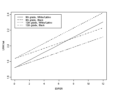
Fig. 5.2, p. 150. Log wage trajectories for four prototypical dropouts from model C.
exper.seq <- seq(0, 12)
fixef.c <- fixef(model.c)
x.w9 <- fixef.c[[1]] + fixef.c[[2]]*exper.seq
x.w12 <-  fixef.c[[1]] + fixef.c[[2]]*exper.seq + fixef.c[[3]]*3
x.b9 <- fixef.c[[1]] + fixef.c[[2]]*exper.seq + fixef.c[[4]]*exper.seq
x.b12 <- fixef.c[[1]] + fixef.c[[2]]*exper.seq + fixef.c[[3]]*3 +
         fixef.c[[4]]*exper.seq
plot(exper.seq, x.w9, ylim=c(1.6, 2.4), ylab="LNW.hat", xlab="EXPER", type="l", lwd=2)
lines(exper.seq, x.w12, lty=3)
lines(exper.seq, x.b9, lty=4, lwd=2)
lines(exper.seq, x.b12, lty=5)
legend(0, 2.4, c("9th grade, White/Latino", "9th grade, Black",
       "12th grade, White/Latino", "12th grade, Black"), lty=c(1, 4, 3, 5))
Inputting the small wages data set.
wages.small <- read.table("https://stats.idre.ucla.edu/stat/r/examples/alda/data/wages_small_pp.txt", header=T, sep=",")
Table 5.5, p. 154.
#Model A
model.a <- lme(lnw~exper+hcg.9+exper:black, wages.small, random= ~exper|id, method="ML")
summary(model.a)

Linear mixed-effects model fit by maximum likelihood
 Data: wages.small
       AIC      BIC    logLik
  299.8772 328.2698 -141.9386

Random effects:
 Formula: ~exper | id
 Structure: General positive-definite, Log-Cholesky parametrization
            StdDev       Corr
(Intercept) 2.902591e-01 (Intr)
exper       1.924436e-05 0
Residual    3.388214e-01

Fixed effects: lnw ~ exper + hcg.9 + exper:black
                 Value  Std.Error  DF  t-value p-value
(Intercept)  1.7373442 0.04812692 131 36.09921  0.0000
exper        0.0517798 0.02109799 131  2.45425  0.0154
hcg.9        0.0457585 0.02468875 122  1.85342  0.0662
exper:black -0.0600723 0.03485043 131 -1.72372  0.0871
 Correlation:
            (Intr) exper  hcg.9
exper       -0.614
hcg.9        0.051 -0.135
exper:black -0.130 -0.294  0.024

Standardized Within-Group Residuals:
        Min          Q1         Med          Q3         Max
-2.42021834 -0.47223444 -0.02901367  0.41970660  4.24393911

Number of Observations: 257
Number of Groups: 124
Inputting the unemployment data set.
unemployment <- read.table("https://stats.idre.ucla.edu/stat/r/examples/alda/data/unemployment_pp.txt", header=T, sep=","
Table 5.6, p. 161.
unemployment[unemployment$id %in% c(7589, 55697, 67641, 65441, 53782),]

       id     months cesd unemp
212  7589  1.3141684   36     1
213  7589  5.0924025   40     1
214  7589 11.7946612   39     1
454 53782  0.4271047   22     1
455 53782  4.2381930   15     0
456 53782 11.0718686   21     1
504 55697  1.3470226    7     1
505 55697  5.7823409    4     1
623 65441  1.0841889   27     1
624 65441  4.6981520   15     1
625 65441 11.2689938    7     0
647 67641  0.3285421   32     1
648 67641  4.1067762    9     0
649 67641 10.9404517   10     0
Table 5.7, p. 163.
#Model A
model.a <- lme(cesd ~ months, unemployment, random= ~months|id, method="ML")
summary(model.a)

Linear mixed-effects model fit by maximum likelihood
 Data: unemployment
       AIC      BIC    logLik
  5145.137 5172.217 -2566.569

Random effects:
 Formula: ~months | id
 Structure: General positive-definite, Log-Cholesky parametrization
            StdDev    Corr
(Intercept) 9.3192519 (Intr)
months      0.5958468 -0.551
Residual    8.2975997

Fixed effects: cesd ~ months
                Value Std.Error  DF   t-value p-value
(Intercept) 17.669363 0.7767173 419 22.748768       0
months      -0.421994 0.0831023 419 -5.078006       0
 Correlation:
       (Intr)
months -0.632

Standardized Within-Group Residuals:
       Min         Q1        Med         Q3        Max
-1.9978128 -0.5415801 -0.1608097  0.4454676  3.5519839

Number of Observations: 674
Number of Groups: 254

#Model B
model.b <- update(model.a, cesd~months+unemp)
summary(model.b)

Linear mixed-effects model fit by maximum likelihood
 Data: unemployment
       AIC      BIC    logLik
  5121.603 5153.196 -2553.802

Random effects:
 Formula: ~months | id
 Structure: General positive-definite, Log-Cholesky parametrization
            StdDev    Corr
(Intercept) 9.6705179 (Intr)
months      0.6816912 -0.591
Residual    7.8985868

Fixed effects: cesd ~ months + unemp
                Value Std.Error  DF   t-value p-value
(Intercept) 12.665598 1.2448444 418 10.174443  0.0000
months      -0.201984 0.0935246 418 -2.159683  0.0314
unemp        5.111304 0.9910522 418  5.157451  0.0000
 Correlation:
       (Intr) months
months -0.715
unemp  -0.780  0.459

Standardized Within-Group Residuals:
       Min         Q1        Med         Q3        Max
-1.9609557 -0.5357110 -0.1191791  0.4303300  3.6857126

Number of Observations: 674
Number of Groups: 254

#Model C
model.c <- update(model.b, cesd~months*unemp)
summary(model.c)

Linear mixed-effects model fit by maximum likelihood
 Data: unemployment
       AIC      BIC    logLik
  5119.047 5155.153 -2551.523

Random effects:
 Formula: ~months | id
 Structure: General positive-definite, Log-Cholesky parametrization
            StdDev    Corr
(Intercept) 9.6805554 (Intr)
months      0.6717203 -0.596
Residual    7.8759886

Fixed effects: cesd ~ months + unemp + months:unemp
                 Value Std.Error  DF   t-value p-value
(Intercept)   9.616744 1.8949397 417  5.074961  0.0000
months        0.162036 0.1942395 417  0.834207  0.4046
unemp         8.529059 1.8834713 417  4.528372  0.0000
months:unemp -0.465222 0.2178620 417 -2.135398  0.0333
 Correlation:
             (Intr) months unemp
months       -0.888
unemp        -0.911  0.863
months:unemp  0.755 -0.878 -0.852

Standardized Within-Group Residuals:
       Min         Q1        Med         Q3        Max
-2.0039251 -0.5237204 -0.1548188  0.4308929  3.6960920

Number of Observations: 674
Number of Groups: 254

#Model D
model.d <- lme(cesd~unemp+unemp:months, unemployment, random=~unemp+unemp:months|id, control = list(optimizer = "nlm", msMaxIter = 100))
summary(model.d)

Linear mixed-effects model fit by REML
 Data: unemployment
       AIC      BIC    logLik
  5115.584 5160.672 -2547.792

Random effects:
 Formula: ~unemp + unempmonths | id
 Structure: General positive-definite, Log-Cholesky parametrization
            StdDev    Corr
(Intercept) 6.7650112 (Intr) unemp
unemp       6.7760936  0.133
unempmonths 0.8738672  0.120 -0.967
Residual    7.6874318

Fixed effects: cesd ~ unemp + unempmonths
                Value Std.Error  DF   t-value p-value
(Intercept) 11.197931 0.7925828 418 14.128405  0.0000
unemp        6.924134 0.9332866 418  7.419086  0.0000
unempmonths -0.303037 0.1124419 418 -2.695056  0.0073
 Correlation:
            (Intr) unemp
unemp       -0.564
unempmonths -0.072 -0.444

Standardized Within-Group Residuals:
       Min         Q1        Med         Q3        Max
-2.1280241 -0.4893635 -0.1558296  0.4256349  3.7748883

Number of Observations: 674
Number of Groups: 254
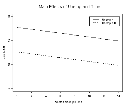
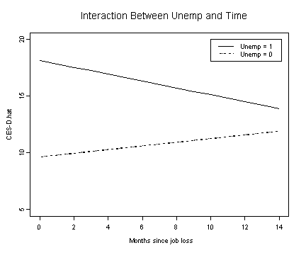
Fig. 5.4, p. 167.
#model B
fixef.b <- fixef(model.b)
months.seq <- seq(0, 14)
unemp.b1 <- fixef.b[[1]] + fixef.b[[2]]*months.seq + fixef.b[[3]]
unemp.b0 <- fixef.b[[1]] + fixef.b[[2]]*months.seq

plot(months.seq, unemp.b1, type="l", ylim=c(5, 20), ylab="CES-D.hat",
     xlab="Months since job loss")
lines(months.seq, unemp.b0, lty=3)
legend(10, 20, c("Unemp = 1", "Unemp = 0"), lty=c(1, 3))
title("Main Effects of Unemp and Time")
#model C
fixef.c <- fixef(model.c)
unemp.c1 <- fixef.c[[1]] + fixef.c[[2]]*months.seq + fixef.c[[3]] +
            fixef.c[[4]]*months.seq
unemp.c0 <- fixef.c[[1]] + fixef.c[[2]]*months.seq

plot(months.seq, unemp.c1, type="l", ylim=c(5, 20), ylab="CES-D.hat",
     xlab="Months since job loss")
lines(months.seq, unemp.c0, lty=3)
legend(10, 20, c("Unemp = 1", "Unemp = 0"), lty=c(1, 3))
title("Interaction Between Unemp and Time"
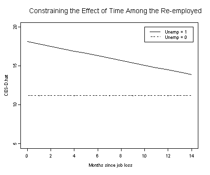
#model D
fixef.d <- fixef(model.d)
unemp.d1 <- fixef.d[[1]] + fixef.d[[3]]*months.seq + fixef.d[[2]]
unemp.d0 <- rep(fixef.d[[1]], 15)

plot(months.seq, unemp.d1, type="l", ylim=c(5, 20), ylab="CES-D.hat",
     xlab="Months since job loss")
lines(months.seq, unemp.d0, lty=3)
legend(10, 20, c("Unemp = 1", "Unemp = 0"), lty=c(1, 3))
title("Constraining the Effect of Time Among the Re-employed")
#Model A
model.a <- lme(lnw~hgc.9+ue.7+exper+exper:black, wages,
           random=~exper|id, method="ML")
summary(model.a)

Linear mixed-effects model fit by maximum likelihood
 Data: wages
       AIC      BIC    logLik
  4848.519 4909.398 -2415.260

Random effects:
 Formula: ~exper | id
 Structure: General positive-definite, Log-Cholesky parametrization
            StdDev     Corr
(Intercept) 0.22502612 (Intr)
exper       0.04039467 -0.32
Residual    0.30788820

Fixed effects: lnw ~ hgc.9 + ue.7 + exper + exper:black
                 Value   Std.Error   DF   t-value p-value
(Intercept)  1.7489885 0.011403780 5511 153.36920   0e+00
hgc.9        0.0400110 0.006365174  886   6.28592   0e+00
ue.7        -0.0119504 0.001792332 5511  -6.66753   0e+00
exper        0.0440539 0.002604399 5511  16.91517   0e+00
exper:black -0.0181832 0.004485454 5511  -4.05382   1e-04
 Correlation:
            (Intr) hgc.9  ue.7   exper
hgc.9        0.086
ue.7        -0.363 -0.039
exper       -0.566 -0.033  0.277
exper:black -0.059 -0.018  0.070 -0.354

Standardized Within-Group Residuals:
        Min          Q1         Med          Q3         Max
-4.34080735 -0.51984995 -0.03652662  0.44253148  6.97854580

Number of Observations: 6402
Number of Groups: 888

#Model B
model.b <- update(model.a, lnw~hgc.9+ue.mean+ue.person.cen+exper+exper:black)
summary(model.b)

Linear mixed-effects model fit by maximum likelihood
 Data: wages
       AIC      BIC    logLik
  4846.978 4914.622 -2413.489

Random effects:
 Formula: ~exper | id
 Structure: General positive-definite, Log-Cholesky parametrization
            StdDev     Corr
(Intercept) 0.22585733 (Intr)
exper       0.04035594 -0.332
Residual    0.30789898

Fixed effects: lnw ~ hgc.9 + ue.mean + ue.person.cen + exper + exper:black
                   Value   Std.Error   DF  t-value p-value
(Intercept)    1.8742603 0.029537336 5511 63.45394       0
hgc.9          0.0401695 0.006353674  885  6.32225       0
ue.mean       -0.0177091 0.003521834  885 -5.02838       0
ue.person.cen -0.0099015 0.002098270 5511 -4.71890       0
exper          0.0450568 0.002651050 5511 16.99581       0
exper:black   -0.0188696 0.004478998 5511 -4.21290       0
 Correlation:
              (Intr) hgc.9  ue.men u.prs. exper
hgc.9          0.058
ue.mean       -0.926 -0.029
ue.person.cen -0.097 -0.027 -0.013
exper         -0.187 -0.031 -0.030  0.334
exper:black   -0.112 -0.019  0.105  0.018 -0.360

Standardized Within-Group Residuals:
        Min          Q1         Med          Q3         Max
-4.34617259 -0.51627687 -0.03591788  0.44100810  7.00029539

Number of Observations: 6402
Number of Groups: 888

#Model C
model.c <- update(model.b, lnw~hgc.9+ue1+ue.centert1+exper+exper:black)
summary(model.c)

Linear mixed-effects model fit by maximum likelihood
 Data: wages
       AIC      BIC    logLik
  4845.842 4913.485 -2412.921

Random effects:
 Formula: ~exper | id
 Structure: General positive-definite, Log-Cholesky parametrization
            StdDev     Corr
(Intercept) 0.22422643 (Intr)
exper       0.04044107 -0.32
Residual    0.30784190

Fixed effects: lnw ~ hgc.9 + ue1 + ue.centert1 + exper + exper:black
                 Value   Std.Error   DF  t-value p-value
(Intercept)  1.8693452 0.026043822 5511 71.77691       0
hgc.9        0.0399276 0.006352135  885  6.28570       0
ue1         -0.0161774 0.002649638  885 -6.10551       0
ue.centert1 -0.0103090 0.001945368 5511 -5.29926       0
exper        0.0447649 0.002626143 5511 17.04588       0
exper:black -0.0183238 0.004486916 5511 -4.08383       0
 Correlation:
            (Intr) hgc.9  ue1    u.cnt1 exper
hgc.9        0.053
ue1         -0.913 -0.022
ue.centert1 -0.335 -0.038  0.335
exper       -0.296 -0.033  0.093  0.302
exper:black -0.069 -0.018  0.058  0.059 -0.353

Standardized Within-Group Residuals:
        Min          Q1         Med          Q3         Max
-4.33611513 -0.51751018 -0.03512461  0.44130726  6.99734177

Number of Observations: 6402
Number of Groups: 888
Inputting the medication data set.
medication <- read.table("https://stats.idre.ucla.edu/stat/r/examples/alda/data/medication_pp.txt", header=T, sep=",")
Table 5.9, p. 182.
medication[c(1:6, 11, 16:21), c(3:8)]

   wave day time.of.day      time   time333    time667
 1    1   0   0.0000000 0.0000000 -3.333333 -6.6666667
 2    2   0   0.3333333 0.3333333 -3.000000 -6.3333333
 3    3   0   0.6666667 0.6666667 -2.666667 -6.0000000
 4    4   1   0.0000000 1.0000000 -2.333333 -5.6666667
 5    5   1   0.3333333 1.3333333 -2.000000 -5.3333333
 6    6   1   0.6666667 1.6666667 -1.666667 -5.0000000
11   11   3   0.3333333 3.3333333  0.000000 -3.3333333
16   16   5   0.0000000 5.0000000  1.666667 -1.6666667
17   17   5   0.3333333 5.3333333  2.000000 -1.3333333
18   19   6   0.0000000 6.0000000  2.666667 -0.6666667
19   20   6   0.3333333 6.3333333  3.000000 -0.3333333
20   21   6   0.6666667 6.6666667  3.333333  0.0000000
21    1   0   0.0000000 0.0000000 -3.333333 -6.6666667
Table 5.10, p. 184.
#Using time (Model A)
model.a <- lme(pos~treat*time, medication, random= ~time|id, method="ML")
summary(model.a)

Linear mixed-effects model fit by maximum likelihood
 Data: medication
       AIC      BIC    logLik
  12696.45 12737.45 -6340.226

Random effects:
 Formula: ~time | id
 Structure: General positive-definite, Log-Cholesky parametrization
            StdDev    Corr
(Intercept) 45.949935 (Intr)
time         7.983475 -0.332
Residual    35.070353

Fixed effects: pos ~ treat * time
                Value Std.Error   DF   t-value p-value
(Intercept) 167.46346  9.341307 1176 17.927198  0.0000
treat        -3.10930 12.352456   62 -0.251715  0.8021
time         -2.41813  1.733646 1176 -1.394822  0.1633
treat:time    5.53681  2.281523 1176  2.426805  0.0154
 Correlation:
           (Intr) treat  time
treat      -0.756
time       -0.404  0.305
treat:time  0.307 -0.408 -0.760

Standardized Within-Group Residuals:
       Min         Q1        Med         Q3        Max
-3.2708599 -0.4899446 -0.1174939  0.4240840  5.6180036

Number of Observations: 1242
Number of Groups: 64

#Using time - 3.33 (Model B)
model.b <- update(model.a, pos~treat*time333)
summary(model.b)

Linear mixed-effects model fit by maximum likelihood
 Data: medication
       AIC      BIC    logLik
  12696.45 12737.45 -6340.226

Random effects:
 Formula: ~time | id
 Structure: General positive-definite, Log-Cholesky parametrization
            StdDev    Corr
(Intercept) 45.949935 (Intr)
time         7.983475 -0.332
Residual    35.070353

Fixed effects: pos ~ treat + time333 + treat:time333
                  Value Std.Error   DF   t-value p-value
(Intercept)   159.40304  8.778656 1176 18.158023  0.0000
treat          15.34674 11.563284   62  1.327196  0.1893
time333        -2.41813  1.733646 1176 -1.394822  0.1633
treat:time333   5.53681  2.281523 1176  2.426805  0.0154
 Correlation:
              (Intr) treat  tim333
treat         -0.759
time333        0.229 -0.174
treat:time333 -0.174  0.222 -0.760

Standardized Within-Group Residuals:
       Min         Q1        Med         Q3        Max
-3.2708599 -0.4899446 -0.1174939  0.4240840  5.6180036

Number of Observations: 1242
Number of Groups: 64

#Using time - 6.67 (Model C)
model.c <- update(model.b, pos~treat*time667)
summary(model.c)

Linear mixed-effects model fit by maximum likelihood
 Data: medication
       AIC      BIC    logLik
  12696.45 12737.45 -6340.226

Random effects:
 Formula: ~time | id
 Structure: General positive-definite, Log-Cholesky parametrization
            StdDev    Corr
(Intercept) 45.949935 (Intr)
time         7.983475 -0.332
Residual    35.070353

Fixed effects: pos ~ treat + time667 + treat:time667
                  Value Std.Error   DF   t-value p-value
(Intercept)   151.34261 11.561102 1176 13.090673  0.0000
treat          33.80278 15.182565   62  2.226421  0.0296
time667        -2.41813  1.733646 1176 -1.394822  0.1633
treat:time667   5.53681  2.281523 1176  2.426805  0.0154
 Correlation:
              (Intr) treat  tim667
treat         -0.761
time667        0.673 -0.513
treat:time667 -0.512  0.670 -0.760

Standardized Within-Group Residuals:
       Min         Q1        Med         Q3        Max
-3.2708599 -0.4899446 -0.1174939  0.4240840  5.6180036

Number of Observations: 1242
Number of Groups: 64
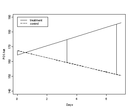
Fig. 5.5, p. 185. Note: The vertical lines reflect the magnitude of the effect of treatment when time is centered at different values.
days.seq <- seq(0, 7)
fixef.a <- fixef(model.a)

trt <- fixef.a[[1]] + fixef.a[[2]] + (fixef.a[[3]]+fixef.a[[4]])*days.seq
cnt <- fixef.a[[1]] + fixef.a[[3]]*days.seq

plot(days.seq, trt, ylim=c(140, 190), xlim=c(0, 7), type="l",
     xlab="Days", ylab="POS.hat")
lines(days.seq, cnt, lty=4)
legend(0, 190, c("treatment", "control"), lty=c(1, 4))
segments(0, fixef.a[[1]] + fixef.a[[3]]*0, 0,
        fixef.a[[1]] + fixef.a[[2]] + (fixef.a[[3]]+fixef.a[[4]])*0)
segments(3.33, fixef.a[[1]] + fixef.a[[3]]*3.33, 3.33,
        fixef.a[[1]] + fixef.a[[2]] + (fixef.a[[3]]+fixef.a[[4]])*3.33)
segments(6.670, fixef.a[[1]] + fixef.a[[3]]*6.670, 6.670,
        fixef.a[[1]] + fixef.a[[2]] + (fixef.a[[3]]+fixef.a[[4]])*6.670)