The R packages needed for this chapter are the survival package and car package. We currently use R 2.0.1 patched version. You may want to make sure that packages on your local machine are up to date. You can perform update in R using update.packages() function.
Table 4.2 on page 119 using data set hmohiv.
hmohiv<-read.table("https://stats.idre.ucla.edu/stat/r/examples/asa/hmohiv.csv", sep=",", header = TRUE)
attach(hmohiv)
library(survival)

drug.coxph
  n= 100
     coef exp(coef) se(coef)    z      p
drug 0.78      2.18    0.242 3.22 0.0013
     exp(coef) exp(-coef) lower .95 upper .95
drug      2.18      0.459      1.36      3.50
Rsquare= 0.097   (max possible= 0.997 )
Likelihood ratio test= 10.2  on 1 df,   p=0.00141
Wald test            = 10.4  on 1 df,   p=0.00130
Score (logrank) test = 10.7  on 1 df,   p=0.00105
Table 4.3, Table 4.4, Table 4.5 and Table 4.6 from page 121 to page 125. We will use the recode function to create a categorical version of age and define it to be a factor variable. Function recode comes with package car.
library(car)
agecat<-recode(age, "20:29='A'; 30:34='B'; 35:39='C';40:54='D'", as.factor=T)
agecat.ph
  n= 100
        coef exp(coef) se(coef)    z       p
agecatB 1.20      3.31    0.451 2.65 8.0e-03
agecatC 1.31      3.72    0.459 2.86 4.2e-03
agecatD 1.86      6.43    0.469 3.96 7.4e-05
        exp(coef) exp(-coef) lower .95 upper .95
agecatB      3.31      0.302      1.37      8.01
agecatC      3.72      0.269      1.51      9.14
agecatD      6.43      0.156      2.56     16.12
Rsquare= 0.178   (max possible= 0.997 )
Likelihood ratio test= 19.6  on 3 df,   p=0.000209
Wald test            = 16.6  on 3 df,   p=0.000875
Score (logrank) test = 18.3  on 3 df,   p=0.000389

names(agecat.ph)

 [1] "coefficients"      "var"               "loglik"
 [4] "score"             "iter"              "linear.predictors"
 [7] "residuals"         "means"             "method"
[10] "n"                 "terms"             "assign"
[13] "wald.test"         "y"                 "formula"
[16] "call"

agecat.ph$var

          [,1]      [,2]      [,3]
[1,] 0.2034328 0.1636590 0.1704751
[2,] 0.1636590 0.2105861 0.1666165
[3,] 0.1704751 0.1666165 0.2202500
Table 4.7 on page 127 using deviation coding scheme. We recode variable agecat so that the first group will be “D” for the last group as the reference. Then we specify that we use the deviation coding via contrasts function.
agecat<-recode(age, "20:29='D'; 30:34='B'; 35:39='C';40:54='A'", as.factor=T)
contrasts(agecat) <- contr.sum(levels(agecat))
agecat.ph <- coxph( Surv(time, censor)~agecat, method="breslow")
summary(agecat.ph)
  n= 100
         coef exp(coef) se(coef)     z       p
agecat1 0.768      2.15    0.209 3.668 0.00024
agecat2 0.104      1.11    0.192 0.543 0.59000
agecat3 0.221      1.25    0.206 1.072 0.28000
        exp(coef) exp(-coef) lower .95 upper .95
agecat1      2.15      0.464     1.430      3.25
agecat2      1.11      0.901     0.762      1.62
agecat3      1.25      0.802     0.833      1.87
Rsquare= 0.178   (max possible= 0.997 )
Likelihood ratio test= 19.6  on 3 df,   p=0.000209
Wald test            = 16.6  on 3 df,   p=0.000875
Score (logrank) test = 18.3  on 3 df,   p=0.000389
Table 4.8 on page 129 using age as a continuous predictor.
age.ph <- coxph( Surv(time, censor)~age, method="breslow")
summary(age.ph)
  n= 100
      coef exp(coef) se(coef)    z     p
age 0.0814      1.08   0.0174 4.67 3e-06
    exp(coef) exp(-coef) lower .95 upper .95
age      1.08      0.922      1.05      1.12
Rsquare= 0.192   (max possible= 0.997 )
Likelihood ratio test= 21.4  on 1 df,   p=3.82e-06
Wald test            = 21.8  on 1 df,   p=3.03e-06
Score (logrank)   test = 22  on 1 df,   p=2.72e-06
Table 4.9 on page 133 using data set uis. We will have to create a variable drug.
rm(list=ls()) #cleaning up
uis<-read.table("https://stats.idre.ucla.edu/stat/r/examples/asa/uis.csv", sep=",", header = TRUE)
attach(uis)
drug<-recode(ivhx, "1=0; 2:3=1")
table(drug)
drug
  0   1
233 377

crude.ph
  n=610 (18 observations deleted due to missing)
      coef exp(coef) se(coef)    z       p
drug 0.326      1.39   0.0946 3.44 0.00057

     exp(coef) exp(-coef) lower .95 upper .95
drug      1.39      0.722      1.15      1.67

Rsquare= 0.02   (max possible= 1 )
Likelihood ratio test= 12.2  on 1 df,   p=0.000476
Wald test            = 11.9  on 1 df,   p=0.000571
Score (logrank) test = 12.0  on 1 df,   p=0.00054
adjust.ph <- coxph( Surv(time, censor)~drug+age, method="breslow")
summary(adjust.ph)
  n=605 (23 observations deleted due to missing)
        coef exp(coef) se(coef)     z       p
drug  0.4394     1.552  0.10072  4.36 1.3e-05
age  -0.0264     0.974  0.00784 -3.37 7.7e-04

     exp(coef) exp(-coef) lower .95 upper .95
drug     1.552      0.644      1.27      1.89
age      0.974      1.027      0.96      0.99

Rsquare= 0.038   (max possible= 1 )
Likelihood ratio test= 23.3  on 2 df,   p=8.65e-06
Wald test            = 23.1  on 2 df,   p=9.72e-06
Score (logrank) test = 23.2  on 2 df,   p=9.21e-06
Table 4.10 on page 135. We first have to make sure that all the models are run on the same observations. To this end, we use function complete.cases to subset the data set.
detach(uis)
touse<-uis[complete.cases(time, censor, treat, age), ]
attach(touse)
crude.ph

  n= 623
        coef exp(coef) se(coef)     z     p
treat -0.220     0.803   0.0893 -2.46 0.014
      exp(coef) exp(-coef) lower .95 upper .95
treat     0.803       1.25     0.674     0.956
Rsquare= 0.01   (max possible= 1 )
Likelihood ratio test= 6.05  on 1 df,   p=0.0139
Wald test            = 6.05  on 1 df,   p=0.0139
Score (logrank) test = 6.07  on 1 df,   p=0.0138

adjust.ph

  n= 623
         coef exp(coef) se(coef)     z     p
treat -0.2230     0.800  0.08933 -2.50 0.013
age   -0.0133     0.987  0.00721 -1.84 0.066
      exp(coef) exp(-coef) lower .95 upper .95
treat     0.800       1.25     0.672     0.953
age       0.987       1.01     0.973     1.001
Rsquare= 0.015   (max possible= 1 )
Likelihood ratio test= 9.48  on 2 df,   p=0.00876
Wald test            = 9.42  on 2 df,   p=0.00903
Score (logrank) test = 9.44  on 2 df,   p=0.00892

inter.ph

  n= 623
              coef exp(coef) se(coef)      z    p
treat      0.52272     1.687   0.4745  1.102 0.27
age       -0.00177     0.998   0.0101 -0.175 0.86
treat:age -0.02319     0.977   0.0145 -1.600 0.11
          exp(coef) exp(-coef) lower .95 upper .95
treat         1.687      0.593     0.665      4.27
age           0.998      1.002     0.979      1.02
treat:age     0.977      1.023     0.950      1.01
Rsquare= 0.019   (max possible= 1 )
Likelihood ratio test= 12.0  on 3 df,   p=0.00724
Wald test            = 11.2  on 3 df,   p=0.0106
Score (logrank) test = 11.3  on 3 df,   p=0.0101
Table 4.11 on page 136 based on the model with interaction of treat and age from previous example. One way of producing Table 4.11 is to simply center age and rerun the model as shown below.
inter.ph <- coxph( Surv(time, censor)~treat+I(age-25)+treat:I(age-25), method="breslow")
summary(inter.ph)
  n= 623
                      coef exp(coef) se(coef)      z    p
treat             -0.05714     0.944   0.1369 -0.417 0.68
I(age - 25)       -0.00177     0.998   0.0101 -0.175 0.86
treat:I(age - 25) -0.02319     0.977   0.0145 -1.600 0.11
                  exp(coef) exp(-coef) lower .95 upper .95
treat                 0.944       1.06     0.722      1.24
I(age - 25)           0.998       1.00     0.979      1.02
treat:I(age - 25)     0.977       1.02     0.950      1.01
Rsquare= 0.019   (max possible= 1 )
Likelihood ratio test= 12.0  on 3 df,   p=0.00724
Wald test            = 11.2  on 3 df,   p=0.0106
Score (logrank) test = 11.3  on 3 df,   p=0.0101
inter.ph <- coxph( Surv(time, censor)~treat+I(age-30)+treat:I(age-30), method="breslow")
summary(inter.ph)
  n= 623
                      coef exp(coef) se(coef)      z     p
treat             -0.17311     0.841   0.0949 -1.825 0.068
I(age - 30)       -0.00177     0.998   0.0101 -0.175 0.860
treat:I(age - 30) -0.02319     0.977   0.0145 -1.600 0.110
                  exp(coef) exp(-coef) lower .95 upper .95
treat                 0.841       1.19     0.698      1.01
I(age - 30)           0.998       1.00     0.979      1.02
treat:I(age - 30)     0.977       1.02     0.950      1.01
Rsquare= 0.019   (max possible= 1 )
Likelihood ratio test= 12.0  on 3 df,   p=0.00724
Wald test            = 11.2  on 3 df,   p=0.0106
Score (logrank) test = 11.3  on 3 df,   p=0.0101
inter.ph <- coxph( Surv(time, censor)~treat+I(age-35)+treat:I(age-35), method="breslow")
summary(inter.ph)
  n= 623
                      coef exp(coef) se(coef)      z      p
treat             -0.28908     0.749   0.0989 -2.924 0.0035
I(age - 35)       -0.00177     0.998   0.0101 -0.175 0.8600
treat:I(age - 35) -0.02319     0.977   0.0145 -1.600 0.1100
                  exp(coef) exp(-coef) lower .95 upper .95
treat                 0.749       1.34     0.617     0.909
I(age - 35)           0.998       1.00     0.979     1.018
treat:I(age - 35)     0.977       1.02     0.950     1.005
Rsquare= 0.019   (max possible= 1 )
Likelihood ratio test= 12.0  on 3 df,   p=0.00724
Wald test            = 11.2  on 3 df,   p=0.0106
Score (logrank) test = 11.3  on 3 df,   p=0.0101
inter.ph <- coxph( Surv(time, censor)~treat+I(age-40)+treat:I(age-40), method="breslow")
summary(inter.ph)
  n= 623
                      coef exp(coef) se(coef)      z      p
treat             -0.40505     0.667   0.1451 -2.791 0.0053
I(age - 40)       -0.00177     0.998   0.0101 -0.175 0.8600
treat:I(age - 40) -0.02319     0.977   0.0145 -1.600 0.1100
                  exp(coef) exp(-coef) lower .95 upper .95
treat                 0.667       1.50     0.502     0.886
I(age - 40)           0.998       1.00     0.979     1.018
treat:I(age - 40)     0.977       1.02     0.950     1.005
Rsquare= 0.019   (max possible= 1 )
Likelihood ratio test= 12.0  on 3 df,   p=0.00724
Wald test            = 11.2  on 3 df,   p=0.0106
Score (logrank) test = 11.3  on 3 df,   p=0.0101
Figure 4.2 on page 139 using data set hmohiv. After running the model, we create a new small data set for prediction purpose.
rm(list=ls()) #cleaning up
library(survival)
hmohiv<-read.table("https://stats.idre.ucla.edu/stat/r/examples/asa/hmohiv.csv", sep=",", header = TRUE)
attach(hmohiv)
fig4_2.ph
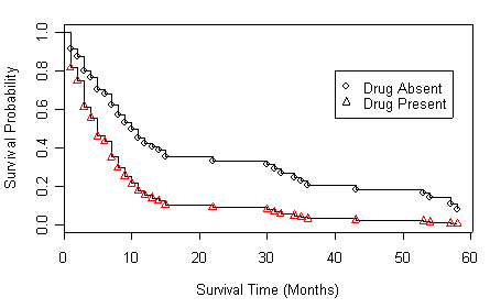
Figure 4.3 on page 141.
Table 4.12 on page 143 with centered age variable.
table4_12.ph <- coxph( Surv(time, censor)~drug+I(age-35), method="breslow")
summary(table4_12.ph)
  n= 100
              coef exp(coef) se(coef)    z       p
drug        0.9414      2.56   0.2555 3.68 2.3e-04
I(age - 35) 0.0915      1.10   0.0185 4.95 7.4e-07
            exp(coef) exp(-coef) lower .95 upper .95
drug             2.56      0.390      1.55      4.23
I(age - 35)      1.10      0.913      1.06      1.14
Rsquare= 0.295   (max possible= 0.997 )
Likelihood ratio test= 35  on 2 df,   p=2.53e-08
Wald test            = 32.5  on 2 df,   p=8.76e-08
Score (logrank) test = 34.3  on 2 df,   p=3.56e-08
Figure 4.4 on page 144 based on the model in the previous example.
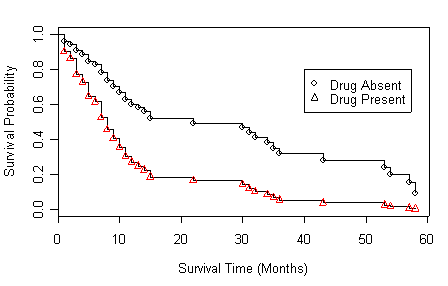
Figure 4.5 on page 146 based on the age-adjusted models at four different age points. We will skip model (b) and (c) since the R code is the same for all of the four panels.
Panel (a) Variable age is centered around 30.
drug.new<-data.frame(drug=c(0,1), age=c(30,30))
age30.ph <- coxph( Surv(time, censor)~drug+I(age-30), method="breslow")
plot(survfit(age30.ph, newdata=drug.new),xlab="Survival Time (Months)",
ylab="Survival Probability")
points(survfit(age30.ph, newdata=drug.new),pch=c(1,2))
legend(40, .8, c("Drug Absent", "Drug Present"), pch=c(1,2))
Panel (d) Variable age is centered around 45.
drug.new<-data.frame(drug=c(0,1), age=c(45,45))
age45.ph <- coxph( Surv(time, censor)~drug+I(age-45), method="breslow")
plot(survfit(age45.ph, newdata=drug.new),xlab="Survival Time (Months)",
ylab="Survival Probability")
points(survfit(age45.ph, newdata=drug.new),pch=c(1,2))
legend(40, .8, c("Drug Absent", "Drug Present"), pch=c(1,2))
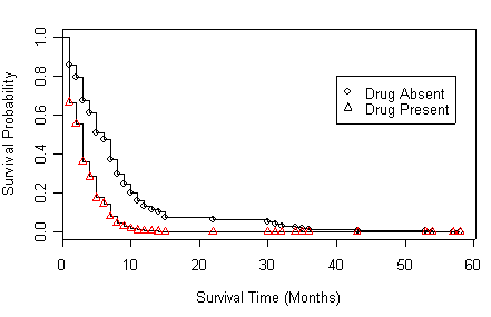
Table 4.13 on page 148 using data set uis.
rm(list=ls()) #cleaning up
library(survival)
uis<-read.table("https://stats.idre.ucla.edu/stat/r/examples/asa/uis.csv", sep=",", header = TRUE)
attach(uis)
drug<-(ivhx==1)
agec<-age-30
ndrugtxc<-ndrugtx-3
full.model <- coxph( Surv(time, censor)~treat+agec+drug+ndrugtxc, method="breslow")
summary(full.model)
  n=593 (35 observations deleted due to missing)
            coef exp(coef) se(coef)     z       p
treat    -0.2271     0.797  0.09158 -2.48 0.01300
agec     -0.0307     0.970  0.00794 -3.87 0.00011
drugTRUE -0.3426     0.710  0.10426 -3.29 0.00100
ndrugtxc  0.0309     1.031  0.00799  3.87 0.00011
         exp(coef) exp(-coef) lower .95 upper .95
treat        0.797       1.25     0.666     0.954
agec         0.970       1.03     0.955     0.985
drugTRUE     0.710       1.41     0.579     0.871
ndrugtxc     1.031       0.97     1.015     1.048
Rsquare= 0.067   (max possible= 1 )
Likelihood ratio test= 41.1  on 4 df,   p=2.57e-08
Wald test            = 43.2  on 4 df,   p=9.26e-09
Score (logrank) test = 43.4  on 4 df,   p=8.38e-09
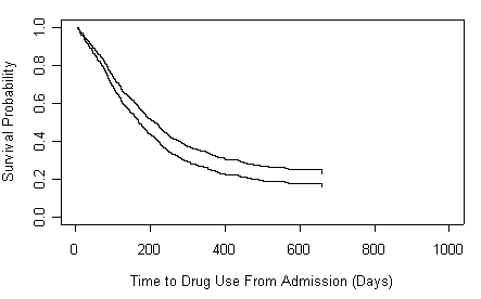
Figure 4.6 on page 148 based on the model in the model above.
fit <- survfit(full.model, conf.type="none")
fit$surv2 <- fit$surv^exp(-0.2271)
plot( fit$time, fit$surv, xlab="Time to Drug Use From Admission (Days)",
      ylab="Survival Probability", ylim=c(0, 1.0), xlim=c(0, 1000), type="s")
points(fit$time, fit$surv2,  type="s")