The R package(s) needed for this chapter is the survival package. We currently use R 2.0.1 patched version. You may want to make sure that packages on your local machine are up to date. You can perform updating in R using update.packages() function.
Table 5.1 on page 166 using data set uis on different covariates.
- Variable hercoc:
rm(list=ls())
library(survival)
uis<-read.table("https://stats.idre.ucla.edu/stat/r/examples/asa/uis.csv", sep=",", header = TRUE)
attach(uis)
hercoc.ph <- coxph( Surv(time, censor) ~ factor(hercoc), method="breslow")
summary(hercoc.ph)
  n=610 (18 observations deleted due to missing)
                   coef exp(coef) se(coef)      z    p
factor(hercoc)2  0.0773     1.080    0.144  0.535 0.59
factor(hercoc)3 -0.2544     0.775    0.135 -1.883 0.06
factor(hercoc)4 -0.1617     0.851    0.130 -1.243 0.21
                exp(coef) exp(-coef) lower .95 upper .95
factor(hercoc)2     1.080      0.926     0.814      1.43
factor(hercoc)3     0.775      1.290     0.595      1.01
factor(hercoc)4     0.851      1.176     0.659      1.10
Rsquare= 0.013   (max possible= 1 )
Likelihood ratio test= 7.76  on 3 df,   p=0.0513
Wald test            = 7.88  on 3 df,   p=0.0486
Score (logrank) test = 7.92  on 3 df,   p=0.0476
survfit( Surv(time, censor) ~ hercoc, uis)
   18 observations deleted due to missing
           n events median 0.95LCL 0.95UCL
hercoc=1 111     92    150     107     198
hercoc=2 114    100    147     110     184
hercoc=3 178    136    185     148     231
hercoc=4 207    165    181     155     220
- Variable ivhx:
detach()
ivhx.ph<-coxph( Surv(time, censor) ~ factor(ivhx), data=uis, method="breslow")
summary(ivhx.ph)
  n=610 (18 observations deleted due to missing)
               coef exp(coef) se(coef)    z       p
factor(ivhx)2 0.195      1.22    0.129 1.52 0.13000
factor(ivhx)3 0.385      1.47    0.101 3.80 0.00014
              exp(coef) exp(-coef) lower .95 upper .95
factor(ivhx)2      1.22      0.822     0.945      1.56
factor(ivhx)3      1.47      0.680     1.205      1.79
Rsquare= 0.024   (max possible= 1 )
Likelihood ratio test= 14.6  on 2 df,   p=0.000663
Wald test            = 14.5  on 2 df,   p=0.000705
Score (logrank) test = 14.7  on 2 df,   p=0.000654
survfit( Surv(time, censor) ~ ivhx, uis)
   18 observations deleted due to missing
         n events median 0.95LCL 0.95UCL
ivhx=1 233    173    194     175     231
ivhx=2 115     93    170     130     231
ivhx=3 262    227    148     115     168
- Variable race:
race.ph<-coxph( Surv(time, censor) ~ factor(race), uis, method="breslow")
summary(race.ph)
  n=622 (6 observations deleted due to missing)
                coef exp(coef) se(coef)     z      p
factor(race)1 -0.284     0.753    0.106 -2.68 0.0073
              exp(coef) exp(-coef) lower .95 upper .95
factor(race)1     0.753       1.33     0.611     0.926
Rsquare= 0.012   (max possible= 1 )
Likelihood ratio test= 7.57  on 1 df,   p=0.00593
Wald test            = 7.21  on 1 df,   p=0.00726
Score (logrank) test = 7.26  on 1 df,   p=0.00706
stci.hl(50, uis, subset=race==0)
     quantile time cie.lower cie.upper
[1,]       50  152       124       174
stci.hl(50, uis, subset=race==1)
     quantile time cie.lower cie.upper
[1,]       50  193       162       232
- Variable treat:
treat.ph<-coxph( Surv(time, censor) ~ factor(treat), uis, method="breslow")
summary(treat.ph)
  n= 628
                 coef exp(coef) se(coef)     z      p
factor(treat)1 -0.231     0.794    0.089 -2.60 0.0094
               exp(coef) exp(-coef) lower .95 upper .95
factor(treat)1     0.794       1.26     0.667     0.945
Rsquare= 0.011   (max possible= 1 )
Likelihood ratio test= 6.75  on 1 df,   p=0.00937
Wald test            = 6.74  on 1 df,   p=0.00941
Score (logrank) test = 6.77  on 1 df,   p=0.00926
survfit( Surv(time, censor) ~ treat, uis)

          n events median 0.95LCL 0.95UCL
treat=0 320    265    132     115     156
treat=1 308    243    192     175     226
Variable site:
site.ph<-coxph( Surv(time, censor) ~ factor(site), uis, method="breslow")
summary(site.ph)
  n= 628
                coef exp(coef) se(coef)     z    p
factor(site)1 -0.151      0.86   0.0986 -1.53 0.13
              exp(coef) exp(-coef) lower .95 upper .95
factor(site)1      0.86       1.16     0.709      1.04
Rsquare= 0.004   (max possible= 1 )
Likelihood ratio test= 2.4   on 1 df,   p=0.121
Wald test            = 2.35  on 1 df,   p=0.125
Score (logrank) test = 2.36  on 1 df,   p=0.125
survfit( Surv(time, censor) ~ site, uis)

         n events median 0.95LCL 0.95UCL
site=0 444    364    156     132     175
site=1 184    144    199     161     232
Variable age:
uis$agecat<-cut(uis$age, c(19, 27, 32,37,56))

agecat.ph<-coxph( Surv(time, censor) ~ agecat, uis, method="breslow")
summary(agecat.ph)
  n=623 (5 observations deleted due to missing)
                         coef exp(coef) se(coef)      z    p
factor(agecat)(27,32]  0.0808     1.084    0.123  0.654 0.51
factor(agecat)(32,37] -0.0658     0.936    0.121 -0.542 0.59
factor(agecat)(37,56] -0.1684     0.845    0.135 -1.247 0.21
                      exp(coef) exp(-coef) lower .95 upper .95
factor(agecat)(27,32]     1.084      0.922     0.851      1.38
factor(agecat)(32,37]     0.936      1.068     0.738      1.19
factor(agecat)(37,56]     0.845      1.183     0.649      1.10
Rsquare= 0.006   (max possible= 1 )
Likelihood ratio test= 3.81  on 3 df,   p=0.282
Wald test            = 3.79  on 3 df,   p=0.285
Score (logrank) test = 3.8   on 3 df,   p=0.284
agecat.surv<-survfit( Surv(time, censor) ~ agecat, uis)
agecat.surv

   5 observations deleted due to missing
                 n events median 0.95LCL 0.95UCL
agecat=(19,27] 158    128    162     122     203
agecat=(27,32] 158    135    148     123     182
agecat=(32,37] 184    145    163     124     216
agecat=(37,56] 123     96    189     168     243
Variable becktoa:
uis$beckt2<-cut(uis$becktota, c(-.5, 9.99,14.9,24.9,55))
beckcat.ph<-coxph( Surv(time, censor) ~ beckt2, uis, method="breslow")
summary(beckcat.ph)
  n=595 (33 observations deleted due to missing)
                    coef exp(coef) se(coef)     z     p
beckt2(9.99,14.9] 0.0752      1.08    0.150 0.502 0.620
beckt2(14.9,24.9] 0.1821      1.20    0.123 1.485 0.140
beckt2(24.9,55]   0.2631      1.30    0.137 1.927 0.054
                  exp(coef) exp(-coef) lower .95 upper .95
beckt2(9.99,14.9]      1.08      0.928     0.804      1.45
beckt2(14.9,24.9]      1.20      0.834     0.943      1.53
beckt2(24.9,55]        1.30      0.769     0.996      1.70
Rsquare= 0.007   (max possible= 1 )
Likelihood ratio test= 4.41  on 3 df,   p=0.221
Wald test            = 4.37  on 3 df,   p=0.225
Score (logrank) test = 4.38  on 3 df,   p=0.223
beckcat.surv<-survfit( Surv(time, censor) ~ beckt2, uis, na.action=na.exclude)
beckcat.surv

   33 observations deleted due to missing
                     n events median 0.95LCL 0.95UCL
beckt2=(-0.5,9.99] 135    104    211     170     248
beckt2=(9.99,14.9] 102     78    170     133     232
beckt2=(14.9,24.9] 226    185    168     139     200
beckt2=(24.9,55]   132    111    146     115     193
Variable ndurgtx:
uis$drugcat<-cut(uis$ndrugtx, c(-.5, 1, 3, 6, 70))
drugcat.ph<-coxph( Surv(time, censor) ~ drugcat, uis, method="breslow")
summary(drugcat.ph)
 n=611 (17 observations deleted due to missing)
                 coef exp(coef) se(coef)      z     p
drugcat(1,3]  -0.0509      0.95    0.123 -0.412 0.680
drugcat(3,6]   0.2661      1.30    0.125  2.134 0.033
drugcat(6,70]  0.3649      1.44    0.127  2.880 0.004
              exp(coef) exp(-coef) lower .95 upper .95
drugcat(1,3]       0.95      1.052     0.746      1.21
drugcat(3,6]       1.30      0.766     1.022      1.67
drugcat(6,70]      1.44      0.694     1.124      1.85
Rsquare= 0.023   (max possible= 1 )
Likelihood ratio test= 14.5  on 3 df,   p=0.0023
Wald test            = 14.7  on 3 df,   p=0.00206
Score (logrank) test = 14.9  on 3 df,   p=0.00192
drugcat.surv<-survfit( Surv(time, censor) ~ drugcat, uis, na.action=na.exclude)
drugcat.surv
Call: survfit(formula = Surv(time, censor) ~ drugcat, data = uis, na.action = na.exclude)
   17 observations deleted due to missing
                   n events median 0.95LCL 0.95UCL
drugcat=(-0.5,1] 183    141    170     143     227
drugcat=(1,3]    165    123    177     162     211
drugcat=(3,6]    138    119    132     106     187
drugcat=(6,70]   125    113    123     110     186
Table 5.2 on page 167 using uis data set.
uis$age5 <- uis$age/5
uis$beck10 <- uis$becktota/10
uis$drug5 <- uis$ndrugtx/5

age5.ph<-coxph( Surv(time, censor) ~ age5, uis, method="breslow")
summary(age5.ph)

  n=623 (5 observations deleted due to missing values)

        coef exp(coef) se(coef)     z     p
age5 -0.0643     0.938   0.0359 -1.79 0.074

     exp(coef) exp(-coef) lower .95 upper .95
age5     0.938       1.07     0.874      1.01

Rsquare= 0.005   (max possible= 1 )
Likelihood ratio test= 3.24 on 1 df,   p=0.0719
Wald test            = 3.2  on 1 df,   p=0.0735
Score (logrank) test = 3.2  on 1 df,   p=0.0735

beck10.ph<-coxph( Surv(time, censor) ~ beck10, uis, method="breslow")
summary(beck10.ph)

  n=595 (33 observations deleted due to missing values)

       coef exp(coef) se(coef)    z    p
beck10 0.11      1.12   0.0472 2.32 0.02

       exp(coef) exp(-coef) lower .95 upper .95
beck10      1.12      0.896      1.02      1.22

Rsquare= 0.009   (max possible= 1 )
Likelihood ratio test= 5.32  on 1 df,   p=0.0211
Wald test            = 5.4   on 1 df,   p=0.0201
Score (logrank) test = 5.41  on 1 df,   p=0.0201

drug5.ph<-coxph( Surv(time, censor) ~ drug5, uis, method="breslow")
summary(drug5.ph)
  n=611 (17 observations deleted due to missing)
       coef exp(coef) se(coef)    z     p
drug5 0.147      1.16   0.0375 3.92 9e-05
      exp(coef) exp(-coef) lower .95 upper .95
drug5      1.16      0.863      1.08      1.25
Rsquare= 0.022   (max possible= 1 )
Likelihood ratio test= 13.4  on 1 df,   p=0.000259
Wald test            = 15.4  on 1 df,   p=8.95e-05
Score (logrank) test = 15.5  on 1 df,   p=8.44e-05
Table 5.3 on page 168 using data set uis.
full.ph <- coxph( Surv(time, censor) ~ age + becktota + ndrugtx + factor(hercoc)
                  + factor(ivhx) + race + treat + site,  uis, method="breslow")
summary(full.ph)
  n=575 (53 observations deleted due to missing)
                    coef exp(coef) se(coef)      z       p
age             -0.02887     0.972  0.00817 -3.533 0.00041
becktota         0.00834     1.008  0.00498  1.677 0.09400
ndrugtx          0.02837     1.029  0.00831  3.416 0.00064
factor(hercoc)2  0.06532     1.067  0.15001  0.435 0.66000
factor(hercoc)3 -0.09362     0.911  0.16547 -0.566 0.57000
factor(hercoc)4  0.02798     1.028  0.16028  0.175 0.86000
factor(ivhx)2    0.17439     1.191  0.13864  1.258 0.21000
factor(ivhx)3    0.28071     1.324  0.14693  1.911 0.05600
race            -0.20289     0.816  0.11669 -1.739 0.08200
treat           -0.23995     0.787  0.09437 -2.543 0.01100
site            -0.10249     0.903  0.10927 -0.938 0.35000
                exp(coef) exp(-coef) lower .95 upper .95
age                 0.972      1.029     0.956     0.987
becktota            1.008      0.992     0.999     1.018
ndrugtx             1.029      0.972     1.012     1.046
factor(hercoc)2     1.067      0.937     0.796     1.432
factor(hercoc)3     0.911      1.098     0.658     1.259
factor(hercoc)4     1.028      0.972     0.751     1.408
factor(ivhx)2       1.191      0.840     0.907     1.562
factor(ivhx)3       1.324      0.755     0.993     1.766
race                0.816      1.225     0.649     1.026
treat               0.787      1.271     0.654     0.946
site                0.903      1.108     0.729     1.118
Rsquare= 0.08   (max possible= 1 )
Likelihood ratio test= 47.9  on 11 df,   p=1.48e-06
Wald test            = 48.8  on 11 df,   p=1.04e-06
Score (logrank) test = 49.4  on 11 df,   p=8.17e-07
Table 5.4 on page 168 using data set uis with smaller model comparing with the previous example.
reduced1.ph <- coxph( Surv(time, censor) ~ age + becktota + ndrugtx +
                      factor(ivhx) + race + treat + site, uis, method="breslow")
summary(reduced1.ph)
  n=575 (53 observations deleted due to missing)
                  coef exp(coef) se(coef)      z       p
age           -0.02822     0.972  0.00817 -3.454 0.00055
becktota       0.00794     1.008  0.00497  1.598 0.11000
ndrugtx        0.02776     1.028  0.00829  3.350 0.00081
factor(ivhx)2  0.19599     1.217  0.13721  1.428 0.15000
factor(ivhx)3  0.33280     1.395  0.11991  2.775 0.00550
race          -0.20925     0.811  0.11589 -1.805 0.07100
treat         -0.23177     0.793  0.09371 -2.473 0.01300
site          -0.09946     0.905  0.10854 -0.916 0.36000
              exp(coef) exp(-coef) lower .95 upper .95
age               0.972      1.029     0.957     0.988
becktota          1.008      0.992     0.998     1.018
ndrugtx           1.028      0.973     1.012     1.045
factor(ivhx)2     1.217      0.822     0.930     1.592
factor(ivhx)3     1.395      0.717     1.103     1.764
race              0.811      1.233     0.646     1.018
treat             0.793      1.261     0.660     0.953
site              0.905      1.105     0.732     1.120
Rsquare= 0.078   (max possible= 1 )
Likelihood ratio test= 46.5  on 8 df,   p=1.90e-07
Wald test            = 47.5  on 8 df,   p=1.24e-07
Score (logrank) test = 48    on 8 df,   p=9.92e-08
Table 5.5 using data set uis, a further reduced model based on the previous example.
uis$ivhx3<-(uis$ivhx==3)
reduced2.ph <- coxph( Surv(time, censor) ~ age + becktota + ndrugtx +
                      ivhx3 + race + treat + site,  uis, method="breslow")
summary(reduced2.ph)
  n=575 (53 observations deleted due to missing)
             coef exp(coef) se(coef)      z      p
age       -0.0262     0.974  0.00805 -3.249 0.0012
becktota   0.0084     1.008  0.00495  1.696 0.0900
ndrugtx    0.0291     1.030  0.00821  3.540 0.0004
ivhx3TRUE  0.2561     1.292  0.10630  2.409 0.0160
race      -0.2245     0.799  0.11527 -1.947 0.0510
treat     -0.2324     0.793  0.09373 -2.480 0.0130
site      -0.0867     0.917  0.10786 -0.804 0.4200
          exp(coef) exp(-coef) lower .95 upper .95
age           0.974      1.026     0.959     0.990
becktota      1.008      0.992     0.999     1.018
ndrugtx       1.030      0.971     1.013     1.046
ivhx3TRUE     1.292      0.774     1.049     1.591
race          0.799      1.252     0.637     1.001
treat         0.793      1.262     0.660     0.952
site          0.917      1.091     0.742     1.133
Rsquare= 0.074   (max possible= 1 )
Likelihood ratio test= 44.5  on 7 df,   p=1.7e-07
Wald test            = 45.5  on 7 df,   p=1.07e-07
Score (logrank) test = 46    on 7 df,   p=8.67e-08
Table 5.6 using data set uis based on the model created in the previous example and the categorical variables created for Table 5.1.
uis$agecat<-cut(uis$age, c(19, 27, 32,37,56))
agecat.ph <- coxph(Surv(time, censor) ~ agecat + becktota + ndrugtx +
                  ivhx3 + site + race + treat, uis, method="breslow")
summary(agecat.ph)
  n=575 (53 observations deleted due to missing)
                  coef exp(coef) se(coef)      z       p
agecat(27,32]  0.03582     1.036  0.13126  0.273 0.78000
agecat(32,37] -0.20940     0.811  0.13003 -1.610 0.11000
agecat(37,56] -0.39059     0.677  0.14996 -2.605 0.00920
becktota       0.00881     1.009  0.00493  1.787 0.07400
ndrugtx        0.02920     1.030  0.00832  3.510 0.00045
ivhx3TRUE      0.24242     1.274  0.10634  2.280 0.02300
site          -0.07911     0.924  0.10849 -0.729 0.47000
race          -0.24549     0.782  0.11618 -2.113 0.03500
treat         -0.22935     0.795  0.09403 -2.439 0.01500
(output omitted.)
uis$beckcat<-cut(uis$becktota, c(-.5, 9.99,14.9,24.9,55))
beckcat.ph <- coxph(Surv(time, censor) ~ age + beckcat + ndrugtx +
                    ivhx3 + site + race + treat, uis, method="breslow")
summary(beckcat.ph)

  n=575 (53 observations deleted due to missing)
                      coef exp(coef) se(coef)      z       p
age                -0.0265     0.974  0.00804 -3.297 0.00098
beckcat(9.99,14.9]  0.0695     1.072  0.15212  0.457 0.65000
beckcat(14.9,24.9]  0.0909     1.095  0.12493  0.728 0.47000
beckcat(24.9,55]    0.2169     1.242  0.13995  1.550 0.12000
ndrugtx             0.0289     1.029  0.00825  3.509 0.00045
ivhx3TRUE           0.2616     1.299  0.10631  2.461 0.01400
site               -0.0920     0.912  0.10782 -0.853 0.39000
race               -0.2254     0.798  0.11549 -1.952 0.05100
treat              -0.2304     0.794  0.09390 -2.453 0.01400
(output omitted)
uis$drugcat<-cut(ndrugtx, c(-.5, 1, 3, 6, 70))
drugcat.ph <- coxph(Surv(time, censor) ~ age + becktota + drugcat +
                    ivhx3 + site + race + treat, uis, method="breslow")
summary(drugcat.ph)

  n=575 (53 observations deleted due to missing)
                  coef exp(coef) se(coef)      z       p
age           -0.02772     0.973  0.00815 -3.402 0.00067
becktota       0.00805     1.008  0.00495  1.626 0.10000
drugcat(1,3]  -0.06951     0.933  0.12911 -0.538 0.59000
drugcat(3,6]   0.25949     1.296  0.13368  1.941 0.05200
drugcat(6,70]  0.39935     1.491  0.14030  2.846 0.00440
ivhx3TRUE      0.24908     1.283  0.10664  2.336 0.02000
site          -0.08384     0.920  0.10791 -0.777 0.44000
race          -0.22966     0.795  0.11542 -1.990 0.04700
treat         -0.21991     0.803  0.09357 -2.350 0.01900
(output omitted)
Figure 5.1 (a), (b) and (c) based on the models from Table 5.6.
Panel (a) Estimated coefficients for grouped age using the object agecat.ph created in the previous example.
names(agecat.ph)
 [1] "coefficients"      "var"               "loglik"
 [4] "score"             "iter"              "linear.predictors"
 [7] "residuals"         "means"             "method"
[10] "n"                 "terms"             "assign"
[13] "wald.test"         "na.action"         "y"
[16] "formula"           "call"
agecat.ph$coefficients
agecat(27,32] agecat(32,37] agecat(37,56]      becktota       ndrugtx
   0.03582336   -0.20940371   -0.39058778    0.00881022    0.02919603
    ivhx3TRUE          site          race         treat
   0.24241703   -0.07910672   -0.24548561   -0.22934666
age.coeff<-data.frame(agecat.ph$coefficients)[1:3,]
age.plot<-cbind(midpt=c(24, 30.5, 35.5, 47.5), rbind(0, data.frame(age.coeff)))
age.plot
   midpt   age.coeff
1   24.0  0.00000000
11  30.5  0.03582336
2   35.5 -0.20940371
3   47.5 -0.39058778
plot(age.plot[,1], age.plot[,2], ylab="Log Hazard", xlab="Age", type="b")
Panel (b) Estimated coefficients for grouped beck score using the object beckcat.ph created in the previous example.
beckcat.ph$coefficients
               age beckcat(9.99,14.9] beckcat(14.9,24.9]   beckcat(24.9,55]
       -0.02650867         0.06948882         0.09094400         0.21687651
           ndrugtx          ivhx3TRUE               site               race
        0.02894029         0.26163192        -0.09197744        -0.22540640
             treat
       -0.23038130
beck.coeff<-data.frame(beckcat.ph$coefficients)[2:4,]
beck.plot<-cbind(midpt=c(5, 12.5, 20, 40), rbind(0, data.frame(beck.coeff)))
plot(beck.plot[,1], beck.plot[,2], ylab="Log Hazard", xlab="Becktota", type="b")
Panel (c) Estimated coefficients for grouped drug treatments using the object drugcat.ph created in the previous example.
drugcat.ph$coefficients
          age      becktota  drugcat(1,3]  drugcat(3,6] drugcat(6,70]
 -0.027723404   0.008050683  -0.069508432   0.259486831   0.399345037
    ivhx3TRUE          site          race         treat
  0.249076482  -0.083840409  -0.229664884  -0.219909556
drug.coeff<-data.frame(drugcat.ph$coefficients)[3:5,]
drug.plot<-cbind(midpt=c(.5, 2.5, 5.0, 23.5), rbind(0, data.frame(drug.coeff)))
drug.plot
   midpt  drug.coeff
1    0.5  0.00000000
11   2.5 -0.06950843
2    5.0  0.25948683
3   23.5  0.39934504
plot(drug.plot[,1], drug.plot[,2], ylab="Log Hazard", xlab="NDRUGTX", type="b")
Figure 5.1 (d) on page 171 and Table 5.7 on page 172 using data set uis and fractional polynomials for ndrugtx. Currently (3/18/05), package mfp does multiple fractional polynomials in regression models, including cox models. You can download the package by “install.packages(“mfp”)” assuming that your machine is connected to the internet. Unlike Stata’s fracpoly command, function mfp in R does not automatically transform variables into desirable forms. For example, if a variable takes value zero sometimes, then negative power is not being used, thus restricting some possible better transformation. In this example, variable ndrugtx takes value zero sometimes, we will apply mfp on a transformed variable.
rm(list=ls())
library(survival)
library(mfp)
uis<-read.table("https://stats.idre.ucla.edu/stat/r/examples/asa/uis.csv", sep=",", header = TRUE)
uis$ivhx3<-(uis$ivhx==3)
uis$nx<-10/(uis$ndrugtx+1)
attach(uis)
uis$ok<-complete.cases(uis$age, uis$becktota, uis$nx, uis$ivhx3, uis$site, uis$race, uis$treat)
to.uis<-uis[ok,]
# Not in the mdoel
a.ph<- coxph(Surv(time, censor) ~ age + becktota + ivhx3 + site + race + treat,
                                  to.uis, method="breslow")
2*a.ph$loglik
[1] -5327.970 -5294.497

# Linear term
alin<- coxph(Surv(time, censor) ~ ndrugtx +  age+ becktota + ivhx3 + site + race + treat,
                                  to.uis, method="breslow")
2*alin$loglik
[1] -5327.970 -5283.459
# J = 1 (2 df)
a2<- mfp(Surv(time, censor) ~fp(nx, df=2) +  age+ becktota + ivhx3 + site + race + treat,
                             family = cox, data = to.uis)
a2$dev
[1] 5281.24
a2$powers
          power1 power2
site         1.0     NA
nx          -0.5     NA
becktota     1.0     NA
race         1.0     NA
treat        1.0     NA
ivhx3TRUE    1.0     NA
age          1.0     NA
# J = 2 (4 df)
a4<- mfp(Surv(time, censor) ~fp(nx, df=4) +  age+ becktota + ivhx3 + site + race + treat,
                             family = cox, data = to.uis)
a4$powers
          power1 power2
site           1     NA
nx             1      1
becktota       1     NA
race           1     NA
treat          1     NA
ivhx3TRUE      1     NA
age            1     NA
a4$dev
[1] 5274.678
Now we are ready to create the plot (d) of Figure 5.1 based on object a4.
names(a4)
 [1] "coefficients"      "var"               "loglik"
 [4] "score"             "iter"              "linear.predictors"
 [7] "residuals"         "means"             "method"
[10] "x"                 "powers"            "pvalues"
[13] "scale"             "df.initial"        "df.final"
[16] "dev"               "dev.lin"           "dev.null"
[19] "fptable"           "n"                 "family"
[22] "wald.test"         "X"                 "y"
[25] "terms"             "call"

head(a4$x)
  site.1     nx.1      nx.2 becktota.1 race.1 treat.1 ivhx3TRUE.1 age.1
1      0 5.000000 8.0471896       9.00      0       1           1    39
2      0 1.111111 0.1170672      34.00      0       1           0    33
3      0 2.500000 2.2907268      10.00      0       1           1    33
4      0 5.000000 8.0471896      20.00      0       0           1    32
5      0 1.666667 0.8513760       5.00      1       1           0    24
6      0 5.000000 8.0471896      32.55      0       1           1    30
y<-a4$x[,2]*(-0.52360) + a4$x[,3]*0.19505
f51.d<-cbind(x=to.uis$ndrugtx, y)
f51.d<-f51.d[order(f51.d$x),]
par(cex=.8)
plot(f51.d$x, f51.d$y, type="l", xlab="NDRUGTX", ylab="Log Hazard")
Table 5.8 on page 174 based on the fractional polynomial model in previous example.
a4
Call:
mfp(formula = Surv(time, censor) ~ fp(nx, df = 4) + age + becktota +
    ivhx3 + site + race + treat, data = to.uis, family = cox)
                coef exp(coef) se(coef)     z       p
site.1      -0.10583     0.900  0.10916 -0.97 3.3e-01
nx.1        -0.52360     0.592  0.12441 -4.21 2.6e-05
nx.2         0.19505     1.215  0.04825  4.04 5.3e-05
becktota.1   0.00918     1.009  0.00499  1.84 6.6e-02
race.1      -0.24242     0.785  0.11547 -2.10 3.6e-02
treat.1     -0.21138     0.809  0.09369 -2.26 2.4e-02
ivhx3TRUE.1  0.25911     1.296  0.10802  2.40 1.6e-02
age.1       -0.02820     0.972  0.00813 -3.47 5.2e-04
Likelihood ratio test=51.6 on 8 df, p=1.99e-08 n= 575
Figure 5.2 on page 175 with Martingale residuals and Lowess smoothed residuals. Library Design includes functions for computing different types of residuals for survival models. You may want have to download the package first by install.packages(“Design”).
Panel (a) Martingale residuals and Lowess smoothed residuals.
detach(uis)
attach(to.uis)
age.ph <- coxph( Surv(time, censor) ~ becktota + ndrugtx + ivhx3
                + race + treat + site,  to.uis, method="breslow")
to.uis$resid<- residuals(age.ph, type="martingale", data=to.uis)
plot(to.uis$age, to.uis$resid, xlab="Age",ylab="Martingale Residuals")
lines(lowess(to.uis$age, to.uis$resid))
Panel (b) Log (Smoothed Censor/Smoothed Expected) + Beta*age.
Fig. 5.3a, p. 176. The fitted line appears to be approximately linear thus there is no transformation of becktota needed.
becktota.ph <- coxph( Surv(time, censor) ~ age + ndrugtx +
  ivhx3 + race + treat + site,  uis, method="breslow", na.action=na.exclude)
uis$resid <- residuals(becktota.ph, type="martingale")
plot(uis$becktota, uis$resid, xlab="Becktota",ylab="Martingale Residuals", ylim=c(-4, 1.0))
lines(lowess(uis$becktota[!is.na(uis$becktota) & !is.na(uis$resid)],
      uis$resid[!is.na(uis$becktota) & !is.na(uis$resid)]))
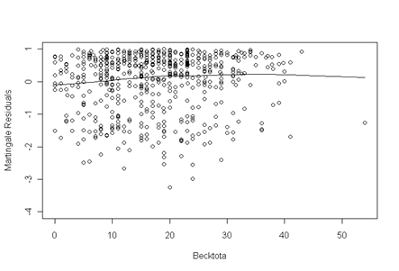
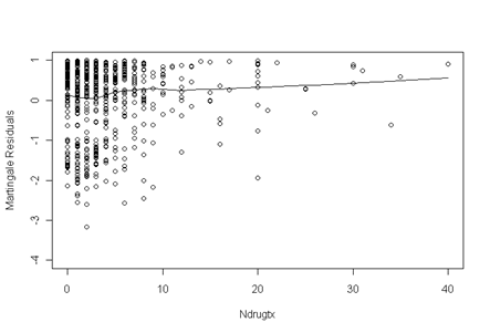
Fig. 5.4a, p. 177. The fitted line has a noticeable squiggle in the beginning which makes us very nervous and it is an indicator that we can’t just include ndrugtx in the model; we should transform it before including it in the final model.
ndrugtx.ph
Creating ndrugfp1 and ndrugfp2, p. 174.
uis$ndrugfp1 <- 1/((uis$ndrugtx+1)/10)
uis$ndrugfp2 <- (1/((uis$ndrugtx+1)/10))*log((uis$ndrugtx+1)/10)
Table 5.8, p. 174.
reduced3.ph <- coxph( Surv(time, censor)~ age + becktota + ndrugfp1 + ndrugfp2 +
   ivhx3 + race + treat + site, uis, method="breslow", na.action=na.exclude)
summary(reduced3.ph)

<output omitted>

  n=575 (53 observations deleted due to missing values)

             coef exp(coef) se(coef)      z        p
     age -0.02815     0.972  0.00813 -3.461 0.000540
becktota  0.00916     1.009  0.00499  1.837 0.066000
ndrugfp1 -0.52284     0.593  0.12441 -4.202 0.000026
ndrugfp2 -0.19478     0.823  0.04825 -4.037 0.000054
   ivhx3  0.25858     1.295  0.10802  2.394 0.017000
    race -0.24220     0.785  0.11547 -2.098 0.036000
   treat -0.21084     0.810  0.09369 -2.250 0.024000
    site -0.10532     0.900  0.10915 -0.965 0.330000

Rsquare= 0.086   (max possible= 1 )
Likelihood ratio test= 51.4  on 8 df,   p=2.17e-008
Wald test            = 51.4  on 8 df,   p=2.17e-008
Score (logrank) test = 52  on 8 df,   p=1.72e-008
Creating the interaction variables, p. 178.
uis$agesite <- uis$age*uis$site
uis$racesite <- uis$race*uis$site
uis$agefp1 <- uis$age*uis$ndrugfp1
uis$agefp2 <- uis$age*uis$ndrugfp2
Table 5.10, p. 179.
interaction.ph <- coxph(formula=Surv(time, censor) ~ age + becktota + + ndrugfp1 + ndrugfp2 +
   ivhx3 + race + treat + site + agesite + racesite + agefp1 + agefp2,
   data=uis, method="breslow", na.action=na.exclude)
summary(interaction.ph)

<output omitted>

  n=575 (53 observations deleted due to missing values)

             coef exp(coef) se(coef)       z       p
     age -0.05431     0.947  0.02803 -1.9372 0.05300
becktota  0.01005     1.010  0.00499  2.0129 0.04400
ndrugfp1 -0.67435     0.509  0.64447 -1.0464 0.30000
ndrugfp2 -0.17217     0.842  0.25234 -0.6823 0.50000
   ivhx3  0.22935     1.258  0.10793  2.1250 0.03400
    race -0.48774     0.614  0.13461 -3.6233 0.00029
   treat -0.24205     0.785  0.09455 -2.5600 0.01000
    site -1.11940     0.326  0.54607 -2.0499 0.04000
 agesite  0.02644     1.027  0.01658  1.5949 0.11000
racesite  0.86274     2.370  0.24810  3.4773 0.00051
  agefp1  0.00163     1.002  0.01945  0.0838 0.93000
  agefp2 -0.00198     0.998  0.00766 -0.2589 0.80000

Rsquare= 0.119   (max possible= 1 )
Likelihood ratio test= 73.1  on 12 df,   p=8.3e-011
Wald test            = 73  on 12 df,   p=8.61e-011
Score (logrank) test = 73.9  on 12 df,   p=5.99e-011
Table 5.11, p. 179.
reducedinter.ph <- coxph(formula=Surv(time, censor) ~ age + becktota + + ndrugfp1 + ndrugfp2 +
 ivhx3 + race + treat + site + agesite + racesite, uis, method="breslow", na.action=na.exclude)
summary(reducedinter.ph)

<output omitted>

  n=575 (53 observations deleted due to missing values)

             coef exp(coef) se(coef)     z        p
     age -0.04138     0.959  0.00991 -4.17 3.0e-005
becktota  0.00874     1.009  0.00497  1.76 7.8e-002
ndrugfp1 -0.57473     0.563  0.12519 -4.59 4.4e-006
ndrugfp2 -0.21470     0.807  0.04859 -4.42 9.9e-006
   ivhx3  0.22776     1.256  0.10857  2.10 3.6e-002
    race -0.46661     0.627  0.13475 -3.46 5.3e-004
   treat -0.24667     0.781  0.09434 -2.61 8.9e-003
    site -1.31517     0.268  0.53143 -2.47 1.3e-002
 agesite  0.03235     1.033  0.01608  2.01 4.4e-002
racesite  0.85014     2.340  0.24774  3.43 6.0e-004

Rsquare= 0.11   (max possible= 1 )
Likelihood ratio test= 67.1  on 10 df,   p=1.58e-010
Wald test            = 66.5  on 10 df,   p=2.07e-010
Score (logrank) test = 67.4  on 10 df,   p=1.38e-010