Applied Survival Analysis, Chapter 6

The R package(s) needed for this chapter is the survival package. We currently use R 2.0.1 patched version. You may want to make sure that packages on your local machine are up to date. You can perform updating in R using update.packages() function.

SPLUS program R program

To input the https://stats.idre.ucla.edu/wp-content/uploads/2016/02/uis-1.csv data set in R use the following code which must be executed before running the R program:

>uis <- read.csv("d:/https://stats.idre.ucla.edu/wp-content/uploads/2016/02/uis-1.csv", header=T)

Here is the SPLUS data set uis.

Creating the dummy variables needed for the model in table 5.11, p. 179.

uis$ivhx3[uis$ivhx>0]

The model from table 5.11, p. 179.

table5.11 

  n=575 (53 observations deleted due to missing values)

              coef exp(coef) se(coef)     z        p 
      age -0.04138     0.959  0.00991 -4.17 3.0e-005
 becktota  0.00874     1.009  0.00497  1.76 7.8e-002
 ndrugfp1 -0.57473     0.563  0.12519 -4.59 4.4e-006
 ndrugfp2 -0.21470     0.807  0.04859 -4.42 9.9e-006
    ivhx3  0.22776     1.256  0.10857  2.10 3.6e-002
     race -0.46661     0.627  0.13475 -3.46 5.3e-004
    treat -0.24667     0.781  0.09434 -2.61 8.9e-003
     site -1.31517     0.268  0.53143 -2.47 1.3e-002
 age:site  0.03235     1.033  0.01608  2.01 4.4e-002
race:site  0.85014     2.340  0.24774  3.43 6.0e-004

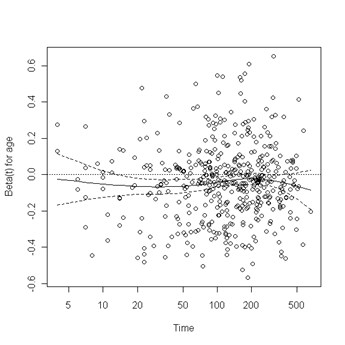
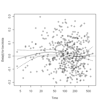
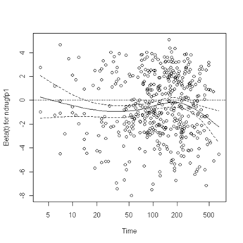
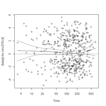
Test of proportionality. The cox.zph function will test proportionality of all the predictors in the model by creating interactions with time using the transformation of time specified in the transform option. In this example we are testing proportionality by looking at the interactions with log(time). The column rho is the Pearson product-moment correlation between the scaled Schoenfeld residuals and log(time) for each covariate. The last row contains the global test for all the interactions tested at once. A p-value less than 0.05 indicates a violation of the proportionality assumption.

#Testing for proportionality.
zph.table5.11 
               rho   chisq     p 
      age  0.03799 0.64964 0.420
 becktota -0.06493 1.83971 0.175
 ndrugfp1 -0.00154 0.00109 0.974
 ndrugfp2  0.00452 0.00943 0.923
    ivhx3 -0.01126 0.05989 0.807
     race  0.04348 0.88737 0.346
    treat  0.06477 1.95669 0.162
     site  0.05065 1.16812 0.280
 age:site -0.05269 1.23768 0.266
race:site -0.00730 0.02479 0.875
   GLOBAL       NA 6.79989 0.744

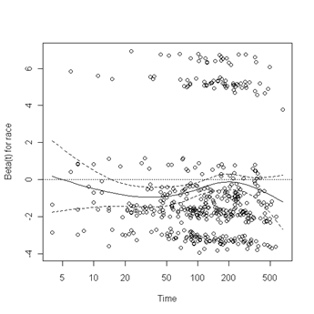
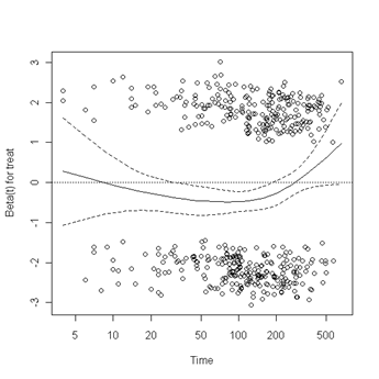
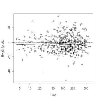
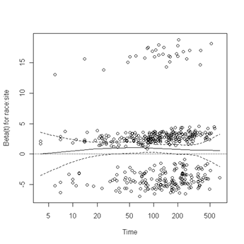
Fig. 6.4, p. 215. The function cox.zph creates a cox.zph object that contains a list of the scaled Schoenfeld residuals. The ordering of the residuals in the list is the same order as the predictors were entered in the cox model. So, the first element of the list corresponds to the scaled Schoenfeld residuals for age, the second element corresponds to the scaled Schoenfeld residuals for ndrugfp1, and so forth. The cox.zph object can be used in a plot function. By specifying a particular element of the list it is possible to generate plots of residuals for individual predictors. Leaving out the list number results in plots for all the predictors being generated at one time. In the plots a non-zero slope is evidence against proportionality. The horizontal line at y=0 has been added for reference.

plot(zph.table5.11[1])
abline(h=0, lty=3)

plot(zph.table5.11[2])
abline(h=0, lty=3)

plot(zph.table5.11[3])
abline(h=0, lty=3)

plot(zph.table5.11[5])
abline(h=0, lty=3)

plot(zph.table5.11[6])
abline(h=0, lty=3)

plot(zph.table5.11[7])
abline(h=0, lty=3)

plot(zph.table5.11[8])
abline(h=0, lty=3)

plot(zph.table5.11[10])
abline(h=0, lty=3)

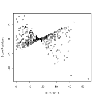
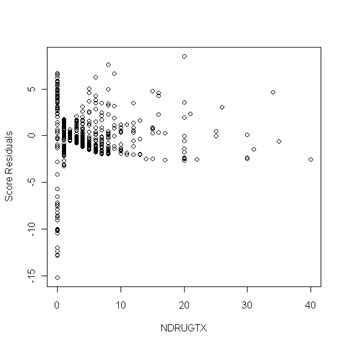
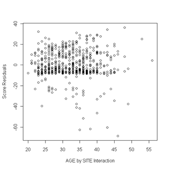
Fig. 6.5, p. 217. First we use the coxph function to obtain a cox model object. Then we can apply the resid function to the cox model object and obtain the score residuals by specifying the option type to equal “score”. The object score is a matrix and the columns of the matrix are the score residuals for the predictors in the cox model. The columns are ordered in the same order as the predictors were entered in the cox model. In other words, column one of the score matrix are the score residual for the predictor age, column two are the score residuals for becktota and so forth. We then generate the plots of the score residuals versus the predictor in order to look for outliers. In general, outliers are points that are isolated from all other points in the graph.

table511.ph

plot(uis$becktota, score[,2], ylab="Score Residuals", xlab="BECKTOTA")

plot(uis$ndrugtx, score[,3], ylab="Score Residuals", xlab="NDRUGTX")

plot(uis$age, score[ ,9], ylab="Score Residuals", xlab="AGE by SITE Interaction")