Note: This page is designed to show the how multilevel model can be done using R and to be able to compare the results with those in the book.
On this page we will use the lmer function which is found in the lme4 package. There are several other possible choices but we will go with lmer.
The data were downloaded in Stata format from here and imported into R using the foreign library from a directory called rdata on the local computer. This page is updated using R 2.11.1 in January, 2011.
library(foreign)
imm10
Table 3.2, page 46. OLS regression lines over 10 schools.
tmp<-by(imm10, schnum, function(x) lm(math ~ homework, data=x))
tmat<-t(sapply(tmp,coef))
tmat

   (Intercept)  homework
1     50.68354 -3.553797
2     49.01229 -2.920123
3     38.75000  7.909091
4     34.39382  5.592664
5     53.93863 -4.718412
6     49.25896 -2.486056
7     59.21022  1.094640
8     36.05535  6.496310
9     38.52000  5.860000
10    37.71392  6.335052
Two equations at the top of page 47.
# get value of public for each school
ptmp<-by(imm10, schnum, function(x) lm(public~1, data=x))
pmat<-as.matrix(sapply(ptmp,coef))
# combine public with intercept and slope
a<-cbind(tmat,pmat)
a

   (Intercept)  homework
1     50.68354 -3.553797 1
2     49.01229 -2.920123 1
3     38.75000  7.909091 1
4     34.39382  5.592664 1
5     53.93863 -4.718412 1
6     49.25896 -2.486056 1
7     59.21022  1.094640 0
8     36.05535  6.496310 1
9     38.52000  5.860000 1
10    37.71392  6.335052 1

summary(lm(a[,1]~a[,3]))

Call:
lm(formula = a[, 1] ~ a[, 3])

Residuals:
   Min     1Q Median     3Q    Max
-8.754 -5.232 -2.199  6.050 10.791

Coefficients:
            Estimate Std. Error t value Pr(>|t|)
(Intercept)   59.210      7.435   7.964 4.51e-05
a[, 3]       -16.063      7.837  -2.050   0.0745

Residual standard error: 7.435 on 8 degrees of freedom
Multiple R-squared: 0.3443,	Adjusted R-squared: 0.2624
F-statistic: 4.201 on 1 and 8 DF,  p-value: 0.07455

summary(lm(a[,2]~a[,3]))

Call:
lm(formula = a[, 2] ~ a[, 3])

Residuals:
   Min     1Q Median     3Q    Max
-6.776 -4.869  1.768  4.159  5.852

Coefficients:
            Estimate Std. Error t value Pr(>|t|)
(Intercept)   1.0946     5.2680   0.208    0.841
a[, 3]        0.9626     5.5530   0.173    0.867

Residual standard error: 5.268 on 8 degrees of freedom
Multiple R-squared: 0.003742,	Adjusted R-squared: -0.1208
F-statistic: 0.03005 on 1 and 8 DF,  p-value: 0.8667
Equation near bottom of page 47 and Table 3.3.
library(lme4)
lmer(math ~ homework + (homework|schnum), REML=FALSE)
Linear mixed model fit by maximum likelihood
Formula: math ~ homework + (homework | schnum)
  AIC  BIC logLik deviance REMLdev
 1781 1803 -884.7     1769    1764
Random effects:
 Groups   Name        Variance Std.Dev. Corr
 schnum   (Intercept) 61.806   7.8617
          homework    19.979   4.4697   -0.804
 Residual             43.067   6.5625
Number of obs: 260, groups: schnum, 10

Fixed effects:
            Estimate Std. Error t value
(Intercept)   44.773      2.603  17.199
homework       2.049      1.472   1.391

Correlation of Fixed Effects:
         (Intr)
homework -0.803
Equation near bottom of page 49 and Table 3.4.
lmer(math ~ homework + public + (homework|schnum), REML=FALSE)
Linear mixed model fit by maximum likelihood
Formula: math ~ homework + public + (homework | schnum)
  AIC  BIC logLik deviance REMLdev
 1765 1790 -875.4     1751    1744
Random effects:
 Groups   Name        Variance Std.Dev. Corr
 schnum   (Intercept) 40.677   6.3778
          homework    21.683   4.6565   -0.982
 Residual             42.955   6.5540
Number of obs: 260, groups: schnum, 10

Fixed effects:
            Estimate Std. Error t value
(Intercept)   58.056      2.695  21.546
homework       1.941      1.525   1.273
public       -14.651      1.831  -8.000

Correlation of Fixed Effects:
         (Intr) homwrk
homework -0.772
public   -0.602  0.010
Equation at the bottom of page 50 and Table 3.5. The negative value for the interaction coefficient in the book is probably a typo error, it should be positive.
lmer(math ~ homework + public + homework:public + (homework|schnum), REML=FALSE)

Linear mixed model fit by maximum likelihood
Formula: math ~ homework + public + homework:public + (homework | schnum)
  AIC  BIC logLik deviance REMLdev
 1767 1795 -875.4     1751    1739
Random effects:
 Groups   Name        Variance Std.Dev. Corr
 schnum   (Intercept) 40.503   6.3642
          homework    21.577   4.6451   -0.982
 Residual             42.954   6.5540
Number of obs: 260, groups: schnum, 10

Fixed effects:
                Estimate Std. Error t value
(Intercept)      59.2102     6.5976   8.975
homework          1.0946     4.6688   0.234
public          -15.9419     6.9775  -2.285
homework:public   0.9472     4.9385   0.192

Correlation of Fixed Effects:
            (Intr) homwrk public
homework    -0.966
public      -0.946  0.913
homwrk:pblc  0.913 -0.945 -0.965
Table 3.6, page 52.
# quietly rerun model from page 47
m1<-lmer(math ~ homework + (homework|schnum), REML=FALSE)

# random intercepts and slopes for each school
rcoef<-coef(m1)
rcoef
$schnum
   (Intercept)  homework
1     50.27101 -3.143116
2     48.88642 -2.753799
3     39.19512  7.566056
4     35.15670  5.393500
5     53.08124 -3.737865
6     48.58612 -1.765064
7     58.05519  1.336116
8     37.15232  6.059531
9     39.16960  5.430173
10    38.17276  6.101294
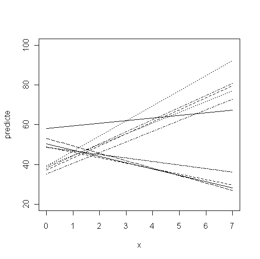
Figure 3.8, page 53.
n<-nrow(rcoef[[1]])
x<-cbind(0, 7)
y<-cbind(seq(1:n), seq(1:n))

y[,1]<-rcoef[[1]][,1]
y[,2]<-rcoef[[1]][,1]+rcoef[[1]][,2]*7

plot(x, y[1,], type="l", ylab="predicte", ylim=c(20,100))
for (i in 2:n){points(x, y[i,], type="l", lty=i)}