The R program for chapter 13.
Since we will only be using the surv data set we will attach it to put it first in the search path.
attach(surv)
We have skipped pages 336-342 for now.
Table 13.3, p. 347.
ct1 <- crosstabs( ~ staget+death)
print(ct1, marginal.totals=F)
ct2 <- crosstabs( ~ perfbl[perfbl != "NA"]+death[perfbl != "NA"])
print(ct2, marginal.totals=F)
ct3 <- crosstabs( ~ treat+death)
print(ct3, marginal.totals=F)
ct4 <- crosstabs( ~ poinf[poinf != "NA"]+death[poinf != "NA"])
print(ct4, marginal.totals=F)

401 cases in table
+----------+
|N         |
|N/RowTotal|
|N/ColTotal|
|N/Total   |
+----------+
staget |death
       |0      |1      |
-------+-------+-------+
0      |122    | 91    |
       |0.57   |0.43   |
       |0.62   |0.45   |
       |0.3    |0.23   |
-------+-------+-------+
1      | 75    |113    |
       |0.4    |0.6    |
       |0.38   |0.55   |
       |0.19   |0.28   |
-------+-------+-------+
Test for independence of all factors
	Chi^2 = 12.07407 d.f.= 1 (p=0.0005112788)
	Yates' correction not used

perfbl[perfbl != "NA"]|death[perfbl != "NA"]
       |0      |1      |
-------+-------+-------+
0      |174    |163    |
       |0.52   |0.48   |
       |0.89   |0.8    |
       |0.44   |0.41   |
-------+-------+-------+
1      | 22    | 40    |
       |0.35   |0.65   |
       |0.11   |0.2    |
       |0.055  |0.1    |
-------+-------+-------+
Test for independence of all factors
	Chi^2 = 5.463732 d.f.= 1 (p=0.01941514)
	Yates' correction not used

treat  |death
       |0      |1      |
-------+-------+-------+
0      | 99    | 96    |
       |0.51   |0.49   |
       |0.5    |0.47   |
       |0.25   |0.24   |
-------+-------+-------+
1      | 98    |108    |
       |0.48   |0.52   |
       |0.5    |0.53   |
       |0.24   |0.27   |
-------+-------+-------+
Test for independence of all factors
	Chi^2 = 0.409521 d.f.= 1 (p=0.5222127)
	Yates' correction not used

poinf[poinf != "NA"]|death[poinf != "NA"]
       |0      |1      |
-------+-------+-------+
0      |191    |189    |
       |0.5    |0.5    |
       |0.97   |0.93   |
       |0.48   |0.47   |
-------+-------+-------+
1      |  5    | 15    |
       |0.25   |0.75   |
       |0.026  |0.074  |
       |0.012  |0.038  |
-------+-------+-------+
Test for independence of all factors
	Chi^2 = 4.852467 d.f.= 1 (p=0.02760662)
	Yates' correction not used
Table 13.4, p. 348.
Log-linear model results.
surv.weibull <- censorReg( censor(days, death) ~ staget+perfbl+poinf+treat,
                  surv, distritution="weibull", na.action=na.omit)
summary(surv.weibull)

Coefficients:
               Est. Std.Err. 95% LCL 95% UCL z-value p-value
(Intercept)  8.6423    0.158   8.332   8.953  54.563 0.00000
     staget -0.5874    0.157  -0.896  -0.279  -3.733 0.00019
     perfbl -0.5986    0.203  -0.996  -0.201  -2.951 0.00317
      poinf -0.7124    0.309  -1.318  -0.107  -2.306 0.02109
      treat -0.0831    0.155  -0.386   0.220  -0.538 0.59078
Table 13.5, p. 349.
Cox’ model results.
surv.cox <- coxph( Surv(days, death) ~ staget+perfbl+poinf+treat,
                  surv, na.action=na.omit)
summary(surv.cox)

         coef exp(coef) se(coef)     z       p
staget 0.5367      1.71    0.142 3.777 0.00016
perfbl 0.5311      1.70    0.185 2.868 0.00410
 poinf 0.6699      1.95    0.280 2.391 0.01700
 treat 0.0705      1.07    0.142 0.497 0.62000
We have skipped pages 350-354 for now.
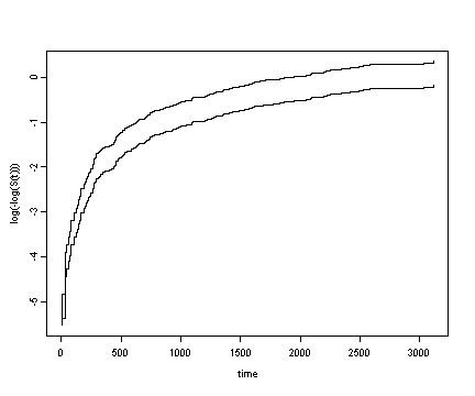
Fig. 13.9, p. 357.
#Obtaining the survival functions.
fit <- survfit(surv.cox, conf.type="none")
fit$surv2 <- fit$surv^exp(.54)

#calculating the log(-log(S(t))
fit$log.surv <- log( -log(fit$surv))
fit$log.surv2 <- log( -log(fit$surv2))

#Plotting
plot( fit$time, fit$log.surv2 , type="s", xlab="time",
      ylab="log(-log(S(t)))" )
points(fit$time, fit$log.surv,  type="s")
Unless you plan to continue working with the surv data set it is advisable to detach it from being first in the search path.
detach(surv)