A standard bar plot can be a very useful tool, but it is often conveying relatively little information–how one variable varies across some grouping variable. The “data-ink ratio” of such a plot is pretty low. This page will show how to build up from the basic bar plot in R, adding another categorical separation to the summary, confidence intervals to the bars, and labels to the bars themselves.
We will use the hsb2 dataset, looking at mean values of math by ses, then by ses and female.
The basic bar plot
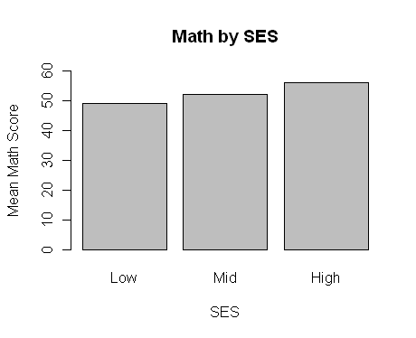
We can construct the basic bar plot using the barplot function in base R. We will include labels on the bars and scale the y axis based on the summary values.
hsb2 <- read.table('https://stats.idre.ucla.edu/stat/r/faq/hsb2.csv', header=T, sep=",")
attach(hsb2)
sesmeans <- tapply(math, ses, mean)
sesmeans
       1        2        3
49.17021 52.21053 56.17241

barplot(sesmeans, main = "Math by SES", xlab = "SES", ylab = "Mean Math Score",
ylim = c(0, 60), names.arg = c("Low", "Mid", "High"))
Adding another grouping variable
We are currently summarizing our data by SES. We might be interested in separating the observations by SES and female. We can create a table of the means of math by these two variables.
femaleses = tapply(math, list(as.factor(ses), as.factor(female)), mean)
femaleses
         0        1
1 47.60000 49.90625
2 53.46809 50.97917
3 54.86207 57.48276
Again we can use barplot for this data. If we have three rows and two columns in the “height” matrix we provide, we can indicate beside = TRUE to create grouped bars. The number of bars per group will be the number of columns and the number of grouped bars will be the number of rows. We can see that transposing femaleses changes the grouping of the bars.
par(mfrow = c(1, 2))
barplot(femaleses, beside = TRUE)
barplot(t(femaleses), beside = TRUE)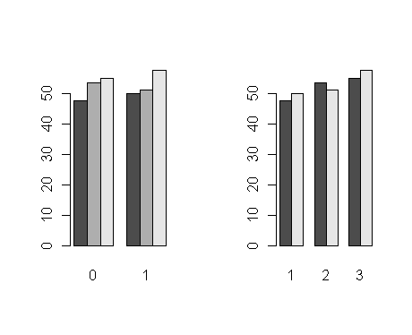
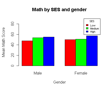
We can add labels and a legend with the code below. We will also specify different colors.
par(mfrow = c(1,1))
barplot(femaleses, beside = TRUE,, main = "Math by SES and gender",
col = c("red", "green", "blue"),
xlab = "Gender", names = c("Male", "Female"),
ylab = "Mean Math Score", legend = c("Low", "Medium", "High"),
args.legend = list(title = "SES", x = "topright", cex = .7), ylim = c(0, 90))
Labeling bars with values
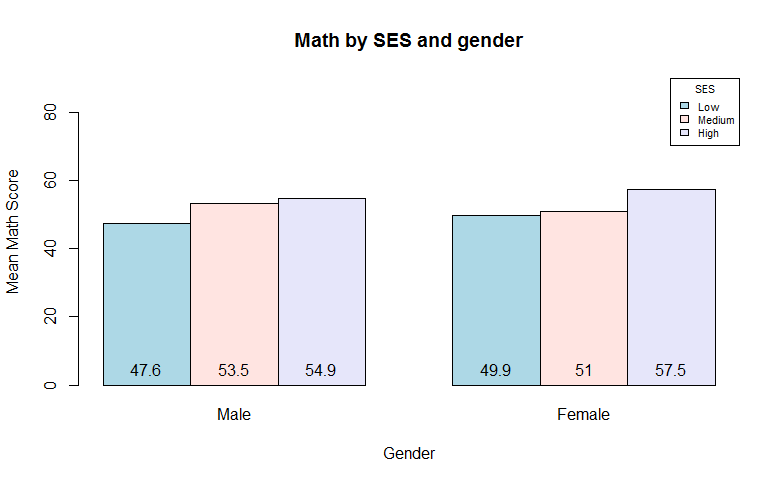
While the levels of the bars indicate which groups have relatively high or low means, we might wish to add the actual mean values to the plot. We can add text to the plot so that the means are printed on the bars. To do this, we will define an object with our bar plot that will be a matrix of the x locations of the bars. Then, we will use the text function to position the heights of the bars (rounded to one decimal) at these x locations and we let y = 0. With pos=3, we describe that we want the text to be placed above the indication locations. We will use lighter colors for the bars to make this added text more readable.
bp <- barplot(femaleses, beside = TRUE, main = "Math by SES and gender",
col = c("lightblue", "mistyrose", "lavender"),
xlab = "Gender", names = c("Male", "Female"),
ylab = "Mean Math Score", legend = c("Low", "Medium", "High"),
args.legend = list(title = "SES", x = "topright", cex = .7), ylim = c(0, 90))
text(bp, 0, round(femaleses, 1),cex=1,pos=3)
Adding confidence bars
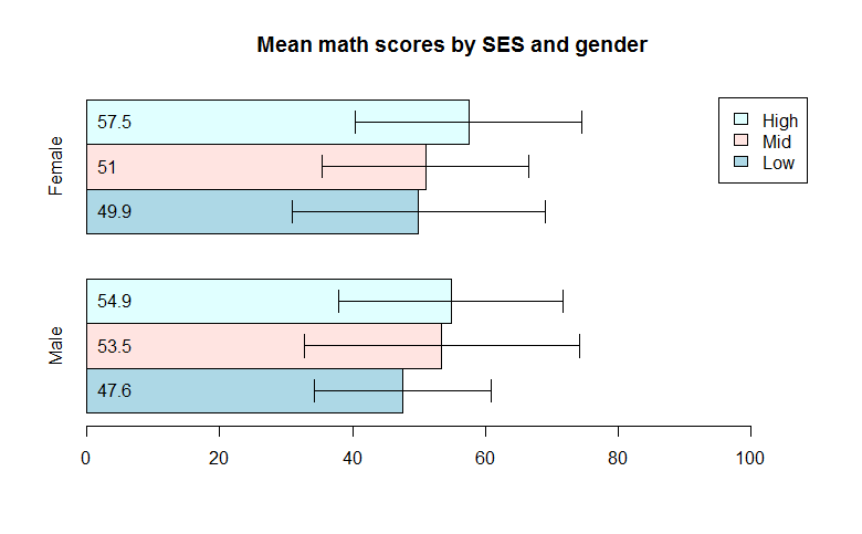
Bar plots are often depicting mean values, but adding some indication of variability can greatly enhance the plot. The gplots package includes an “enhanced bar plot” function called barplot2. We will use this to add confidence intervals to the plot above. There is an argument, plot.ci, that can be indicated as true and then the upper and lower cutoffs are passed as additional arguments. We will also turn the bars sideways, indicating horiz = TRUE.
library(gplots)
mathsd = tapply(math, list(as.factor(ses), as.factor(female)), sd)
upper = femaleses+ 1.96*mathsd
lower = femaleses- 1.96*mathsd
bp <- barplot2(femaleses, beside = TRUE, horiz = TRUE,
names.arg = c("Male", "Female"),plot.ci = TRUE, ci.u = upper, ci.l = lower,
col = c("lightblue", "mistyrose", "lightcyan"), xlim = c(0, 110),
legend = c("Low", "Mid", "High"),main = c("Mean math scores by SES and gender"))
text(0,bp,round(femaleses, 1),cex=1,pos=4)
