How can I do a scatterplot with regression line or any other lines?

R makes it very easy to create a scatterplot and regression line using an lm object created by lm function. We will illustrate this using the hsb2 data file.

hsb2<-read.table("https://stats.idre.ucla.edu/stat/data/hsb2.csv", sep=",", header=T)
head(hsb2)

   id female  race    ses schtyp     prog read write math science socst
1  70   male white    low public  general   57    52   41      47    57
2 121 female white middle public vocation   68    59   53      63    61
3  86   male white   high public  general   44    33   54      58    31
4 141   male white   high public vocation   63    44   47      53    56
5 172   male white middle public academic   47    52   57      53    61
6 113   male white middle public academic   44    52   51      63    61

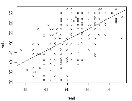
Here we can make a scatterplot of the variables write with read.

	reg1 <- lm(write~read,data=hsb2) 
	summary(reg1)
	
	with(hsb2,plot(read, write))
	abline(reg1)

Image scatte1

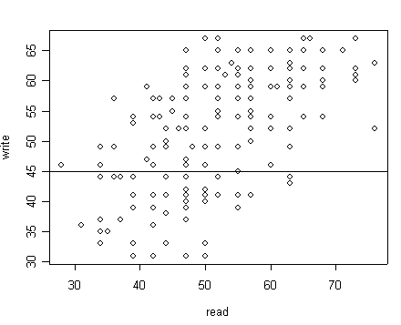
The abline function is actually very powerful. We can add any arbitrary lines using this function. For example, we can add a horizontal line at write = 45 as follows.

	with(hsb2, plot(read, write))
	abline(h=45)

Image scatte2

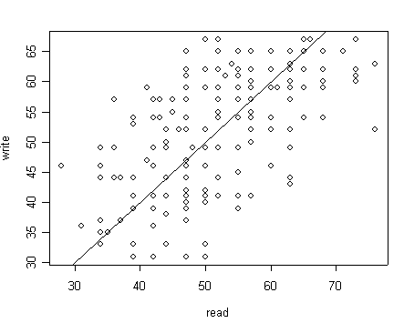
Here is another example where we add a line of 45 degree angle passing through the origin. In this type of syntax, the first parameter is the intercept and the second one the slope.

	with(hsb2,plot(read, write))
	abline(0, 1)