The R package boot allows a user to easily generate bootstrap samples of virtually any statistic that they can calculate in R. From these samples, you can generate estimates of bias, bootstrap confidence intervals, or plots of your bootstrap replicates. We will demonstrate a few of these techniques in this page and you can read more details at its CRAN package page. Before using commands in the boot package, you must first download the package and load it in your workspace. We will be using the hsb2 dataset for all of the examples on this page.
install.packages("boot",dep=TRUE)
library(boot)
hsb2 <- read.table("https://stats.idre.ucla.edu/stat/data/hsb2.csv", sep=",", header=T)
Using the boot command
The boot command executes the resampling of your dataset and calculation of your statistic(s) of interest on these samples. Before calling boot, you need to define a function that will return the statistic(s) that you would like to bootstrap. The first argument passed to the function should be your dataset. The second argument can be an index vector of the observations in your dataset to use or a frequency or weight vector that informs the sampling probabilities. The example below uses the default index vector and assumes we wish to use all of our observations. The statistic of interest here is the correlation coefficient of write and math.
fc <- function(d, i){
	d2 <- d[i,]
	return(cor(d2$write, d2$math))
}
With the function fc defined, we can use the boot command, providing our dataset name, our function, and the number of bootstrap samples to be drawn.
#turn off set.seed() if you want the results to vary
set.seed(626)
bootcorr <- boot(hsb2, fc, R=500)
bootcorr
ORDINARY NONPARAMETRIC BOOTSTRAP

Call:
boot(data = hsb2, statistic = fc, R = 500)


Bootstrap Statistics :
     original       bias    std. error
t1* 0.6174493 -0.001528707  0.04020362
While the printed output for bootcorr is brief, R saves additional information that can be listed:
summary(bootcorr)
          Length Class      Mode
t0          1    -none-     numeric
t         500    -none-     numeric
R           1    -none-     numeric
data       11    data.frame list
seed      626    -none-     numeric
statistic   1    -none-     function
sim         1    -none-     character
call        4    -none-     call
stype       1    -none-     character
strata    200    -none-     numeric
weights   200    -none-     numeric
Knowing the seed value would allow us to replicate this analysis, if needed, and from the t vector and t0, we could calculate the bias and standard error:
mean(bootcorr$t) - bootcorr$t0
[1] -0.001528707
sd(bootcorr$t)
[1] 0.04020362
For using other commands in the boot package, you will often need to provide a “boot” object:
class(bootcorr)
[1] "boot"
Bootstrap confidence intervals and plots
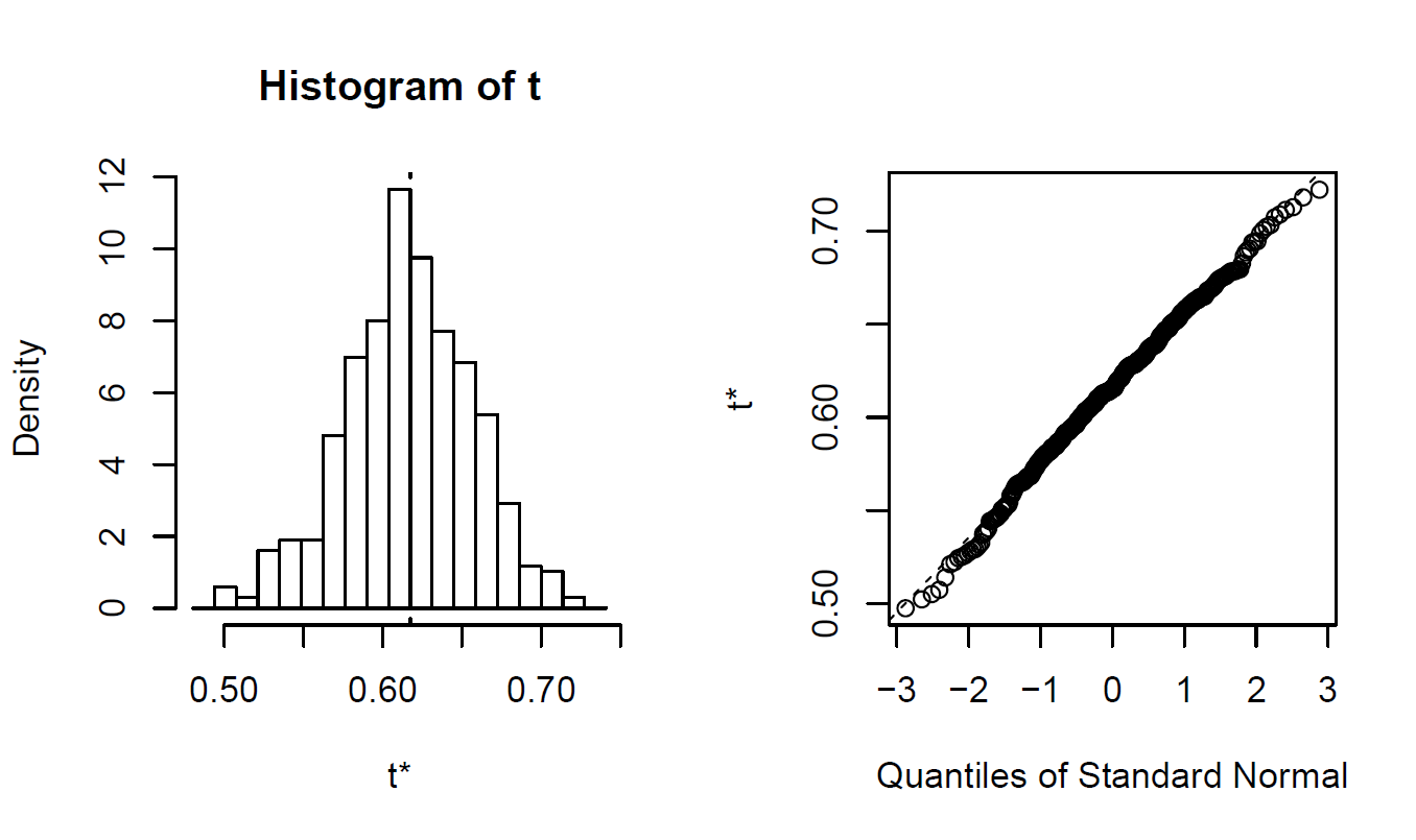
To look at a histogram and normal quantile-quantile plot of your bootstrap estimates, you can use plot with the “boot” object you created. The histogram includes a dotted vertical line indicating the location of the original statistic.
plot(bootcorr)
Using the boot.ci command, you can generate several types of confidence intervals from your bootstrap samples.
boot.ci(boot.out = bootcorr, type = c("norm", "basic", "perc", "bca"))BOOTSTRAP CONFIDENCE INTERVAL CALCULATIONS Based on 500 bootstrap replicates CALL : boot.ci(boot.out = bootcorr, type = c("norm", "basic", "perc", "bca")) Intervals : Level Normal Basic 95% ( 0.5402, 0.6978 ) ( 0.5406, 0.7063 ) Level Percentile BCa 95% ( 0.5286, 0.6943 ) ( 0.5291, 0.6946 ) Calculations and Intervals on Original Scale
Four 95% confidence intervals are presented: normal, basic, percentile, and bias-corrected and accelerated. A fifth type, the studentized intervals, requires variances from each bootstrap sample.
